Part (a)

Implement your accept-reject algorithm and Metropolis-hastings algorithms to get a sample of $10000$ from $Y\sim \mathrm{GAM}(\alpha =2.5,1)$.

# The density function for random variates in the family
# GAM(shape=alpha,rate=1)
dgamma1 <- function(x, alpha) {
    dgamma(x, shape = alpha, rate = 1)
}

# An acceptance-rejection sampling procedure for random variates in the family
# GAM(shape=alpha,rate=1)
accept.reject.rgamma1 <- function(n, alpha) {
    a <- floor(alpha)
    rate <- a/alpha
    q <- (alpha/exp(1))^(a - alpha)
    ys <- vector(length = n)
    for (i in 1:n) {
        repeat {
            y <- sum(rexp(a, rate))  # draw candidate
            if (runif(1) <= q * y^(alpha - a) * exp(y * a/alpha - y)) {
                ys[i] <- y
                break
            }
        }
    }
    ys
}

alpha <- 2.5
m <- 10000
accept.reject.samp <- accept.reject.rgamma1(m, alpha)

# A sampling procedure for random variates in the family
# GAM(shape=alpha,rate=1) using Metropolis-Hastings algorithm
metro.hast.rgamma1 <- function(n, alpha, burn = 0) {
    a <- floor(alpha)
    rate <- a/alpha

    # density for random variates in the family GAM(shape=alpha,rate=1)
    f <- function(x) {
        dgamma(x, shape = alpha, rate = 1)
    }
    g <- function(x) {
        dgamma(x, shape = a, rate = rate)
    }

    m <- n + burn
    ys <- vector(length = m)
    ys[1] <- sum(rexp(a, rate))

    for (i in 2:m) {
        v <- sum(rexp(a, rate))  # draw from g
        u <- ys[i - 1]
        R <- f(v) * g(u)/(f(u) * g(v))
        if (runif(1) <= R) {
            ys[i] <- v
        } else {
            ys[i] <- u
        }
    }
    ys[(burn + 1):m]
}

metro.hast.samp <- metro.hast.rgamma1(m, alpha)

Part (b)

Check on mixing and convergence using plots. Run multiple chain and compute the Gelman-Rubin statistics. You may pick any reasonable burn-in.

We plot the histograms with:

par(mfrow = c(1, 2))
hist(accept.reject.samp, freq = F, breaks = 50, main = "acceptance-rejection")
lines(seq(0.01, 15, by = 0.01), dgamma1(seq(0.01, 15, by = 0.01), alpha), col = "blue",
    lwd = 2)

hist(metro.hast.samp, freq = F, breaks = 50, main = "metropolis-hastings")
lines(seq(0.01, 15, by = 0.01), dgamma1(seq(0.01, 15, by = 0.01), alpha), col = "blue",
    lwd = 2)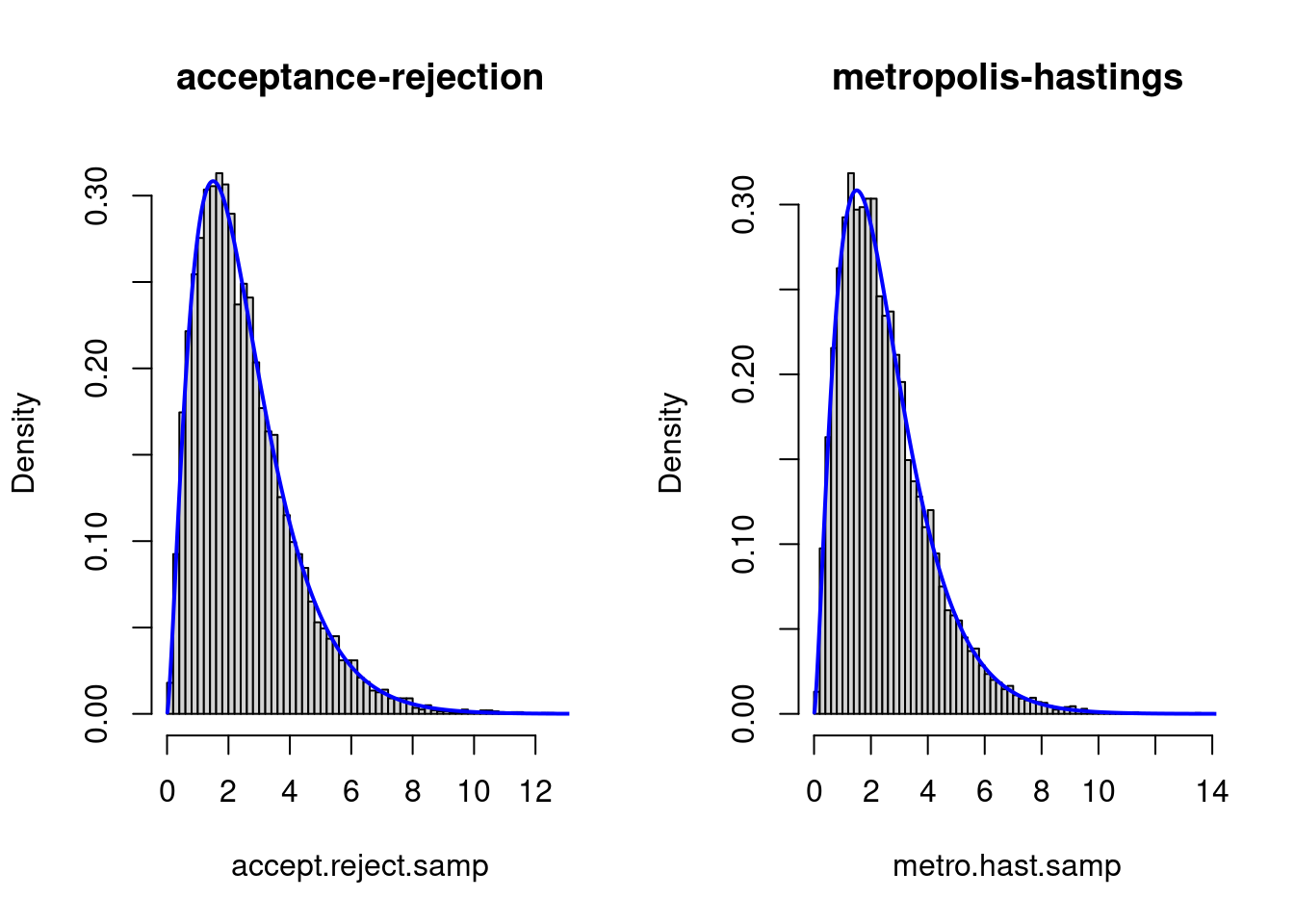

Both samplers seem to be compatible with the density.

We plot the of the Metropolis-Hastings and acceptance-rejection samplers with:

par(mfrow = c(1, 2))
plot(metro.hast.samp, pch = "·", xlab = "t", ylab = "Y", main = "metropolis-hastings")
plot(accept.reject.samp, pch = "·", xlab = "t", ylab = "Y", main = "acceptance-rejection")

Both of these look good, as neither remain at or near the same value for many iterations. They also both quickly move away from their initial values.

We plot the ACFs with:

par(mfrow = c(1, 2))
acf(metro.hast.samp)
acf(accept.reject.samp)

Both samplers seem to have very little autocorrelation. If an uncorrelated sample is extremely important, to be safe, taking every other sample point would probably be sufficient.

We implement the Gelman-Rubin statistic with:

# samps: should be an L x J matrix, where L is the length of the samples and J
# is the number of samples (independent chains).
gelman.rubin <- function(samps) {
    L <- nrow(samps)
    J <- ncol(samps)
    x.bar <- apply(samps, 2, mean)
    B <- var(x.bar) * L
    W <- mean(apply(samps, 2, var))

    ((L - 1)/L * W + B/L)/W
}

Next, we compute Gelman-Rubin statistics on the computed independence chains.

chains <- 1000
samps <- matrix(nrow = m, ncol = chains)
for (i in 1:chains) {
    samps[, i] <- metro.hast.rgamma1(m, alpha, burn = 1000)
}

gelman.rubin.stat <- gelman.rubin(samps)
print(gelman.rubin.stat)

## [1] 1.000009

We see that the Gelman-Rubin statistic is given by $$R=1.0000087.$$

We adopt the rule of thumb that if $\sqrt{R}<1.1$, the burn-in and chain length are sufficient. We compute $\sqrt{R}$ to be $$\sqrt{R}=1.0000044,$$ and thus are satisfied with our burn-in choice and chain length.

Part (c)

Estimate $\mathrm{E}(Y^2)$ using the generated chain. Compare with the estimate you get with acceptance-rejection sampling (Exam 1).

Theoretically, $$\mathrm{E}(Y^2)=\frac{\mathrm{\Gamma }(2+\alpha )}{\mathrm{\Gamma }(\alpha )}=\frac{\mathrm{\Gamma }(4.5)}{\mathrm{\Gamma }(2.5)}=8.75.$$

We estimate $\mathrm{E}(Y^2)$ using the acceptance-rejection and Metropolis-Hastings by taking the square of each element in the samples they generated and then taking the mean:

tab <- matrix(nrow = 2, ncol = 1)
rownames(tab) <- c("acceptance-rejection", "metropolis-hastings")
colnames(tab) <- c("mean")
tab[1] <- c(mean(accept.reject.samp^2))
tab[2] <- c(mean(metro.hast.samp^2))

knitr::kable(data.frame(tab))

Both are quite close to the true value of $8.75$.

Part (a)

Simulate $200$ realizations from the mixture distribution with $\delta =0.7$. Draw a histogram of these data.

We implement the density and sampler for the mixture distribution with:

dmix <- function(x, delta) {
    delta * dnorm(x, 7, 0.5) + (1 - delta) * dnorm(x, 10, 0.5)
}

rmix <- function(n, delta) {
    xs <- vector(length = n)
    for (i in 1:n) {
        xs[i] <- ifelse(runif(1) < delta, rnorm(1, 7, 0.5), rnorm(1, 10, 0.5))
    }
    xs
}

We generate a sample and plot its histogram with:

n <- 200
delta <- 0.7
data <- rmix(n, delta)
hist(data, freq = F)

Part (b)

Now assume $\delta$ is unknown. Implement independence chain MCMC procedure to simulate from the posterior distribution of $\delta$, using your data from part (a).

lmix <- Vectorize(function(delta, xs) {
    if (delta < 0 || delta > 1) {
        return(0)
    }
    p <- 1
    for (x in xs) {
        p <- p * dmix(x, delta)
    }
    p
}, "delta")

logmix <- Vectorize(function(delta, xs) {
    if (delta < 0 || delta > 1) {
        return(-Inf)
    }
    logp <- 0
    for (x in xs) {
        logp <- logp + log(dmix(x, delta))
    }
    logp
}, "delta")

A sample $\{x_t\}$ drawn from the mixture normal with density $\mathrm{dmix}$ is observed with likelihood $\mathrm{lmix}(\delta |\overrightarrow{x})$ with respect to $\delta$ with prior distribution $p(\delta )$. Thus, the posterior distribution is given by $$p(\delta |\overrightarrow{x})\propto p(\delta )\mathrm{lmix}(\delta |\overrightarrow{x}).$$

In the independence chain MCMC, we may use the prior as the proposal density, $f(\delta )=p(\delta |\overrightarrow{x})$ and $g=p$, and thus $$R=\frac{f({\delta }^{\ast })g({\delta }^{(t)})}{f({\delta }^{(t)})g({\delta }^{\ast })}=\frac{p({\delta }^{\ast }|\overrightarrow{x})p({\delta }^{(t)})}{p({\delta }^{(t)}|\overrightarrow{x})p({\delta }^{\ast })}$$ which may be rewritten as $$R=\frac{p({\delta }^{\ast })\mathrm{lmix}({\delta }^{\ast }|\overrightarrow{x})p({\delta }^{(t)})}{p({\delta }^{(t)})\mathrm{lmix}({\delta }^{(t)}|\overrightarrow{x})p({\delta }^{\ast })}=\frac{\mathrm{lmix}({\delta }^{\ast }|\overrightarrow{x})}{\mathrm{lmix}({\delta }^{(t)}|\overrightarrow{x})}.$$

delta.estimator.ic <- function(n, data, delta0 = runif(1), burn = 0) {
    m <- n + burn
    deltas <- vector(length = m)
    deltas[1] <- delta0

    for (i in 2:m) {
        delta <- runif(1)  # draw candidate from prior
        delta.old <- deltas[i - 1]
        log.R <- logmix(delta, data) - logmix(delta.old, data)
        if (log(runif(1)) <= log.R) {
            deltas[i] <- delta
        } else {
            deltas[i] <- delta.old
        }
    }
    deltas[(burn + 1):m]
}

Part (c)

Implement a random walk chain with ${\delta }^{\ast }={\delta }^{(t)}+{ϵ}_t$ with $ϵ\sim \mathrm{UNIF}(-1,1)$.

We observe that ${ϵ}_t\sim \mathrm{UNIF}(-1,1)$ for $t=0,\dots ,t$ are the only random components. Thus, the conditional distribution of ${ϵ}_{t+1}$ given ${ϵ}_t$ is $${ϵ}_{t+1}\sim f({\delta }^{\ast }-{\delta }^{(t)})$$ where $f$ is the density of $\mathrm{UNIF}(-1,1)$.

delta.estimator.rw <- function(n, data, delta0 = runif(1), burn = 0) {
    m <- n + burn
    deltas <- vector(length = m)
    deltas[1] <- delta0
    for (i in 2:m) {
        delta.old <- deltas[i - 1]
        delta <- delta.old + runif(1, -1, 1)
        log.R <- logmix(delta, data) - logmix(delta.old, data)
        if (log(runif(1)) <= log.R) {
            deltas[i] <- delta
        } else {
            deltas[i] <- delta.old
        }
    }
    deltas[(burn + 1):m]
}

Part (d)

Reparameterize the problem letting $U=\log (\delta /(1-\delta ))$ and $U^{\ast }=u(t)+{ϵ}_t$. Implement a random walk chain with $U$ as in Equation (7.8) page 208.

logit <- function(delta) {
    log(delta/(1 - delta))
}
logit.inv <- function(u) {
    exp(u)/(1 + exp(u))
}
logit.inv.J <- function(u) {
    exp(u)/(1 + exp(u))^2
}

delta.estimator.u.rw <- function(n, data, delta0 = runif(1), burn = 0) {
    m <- n + burn
    u <- vector(length = m)
    u[1] <- logit(delta0)
    for (i in 2:m) {
        u.old <- u[i - 1]
        u.star <- u.old + runif(1, -1, 1)
        R <- lmix(logit.inv(u.star), data) * logit.inv.J(u.star)/(lmix(logit.inv(u.old),
            data) * logit.inv.J(u.old))
        if (runif(1) <= R) {
            u[i] <- u.star
        } else {
            u[i] <- u.old
        }
    }
    logit.inv(u[(burn + 1):m])
}

Part (e)

Compare the estimates and convergence behavior of three algorithms.

We do not do a burn-in, since we are interested in seeing how quickly the three methods converge. We only plot chains of length $1000$.

We generate the data sets with:

chain <- 1000
burn <- 0
deltas.ic <- delta.estimator.ic(chain, data, burn = burn)
deltas.rw <- delta.estimator.rw(chain, data, burn = burn)
deltas.u.rw <- delta.estimator.u.rw(chain, data, burn = burn)
tab <- matrix(nrow = 3, ncol = 1)
rownames(tab) <- c("independence chain", "random walk", "reparameterized random walk")
colnames(tab) <- c("mu")
tab[1, ] <- mean(deltas.ic)
tab[2, ] <- mean(deltas.rw)
tab[3, ] <- mean(deltas.u.rw)
knitr::kable(data.frame(tab))

As the table of estimations shows, all three methods provide a good estimate of $\delta$. Next, we consider their convergence and mixing behavior.

We plot the histograms with:

par(mfrow = c(1, 3))
hist(deltas.ic, freq = F, breaks = 50, main = "independence chain")
hist(deltas.rw, freq = F, breaks = 50, main = "random walk")
hist(deltas.u.rw, freq = F, breaks = 50, main = "reparameterized random walk")

The reparameterized random walk metropolis has a histogram that is most compatible with normality, i.e., characteristic bell curve with a mode at $\delta =0.7$. That said, all three histograms arguably satisfy normality with approximately the same mean at $\delta =0.7$.

We plot the sample paths with:

par(mfrow = c(1, 3))
plot(deltas.ic, pch = "·", type = "l", xlab = "t", ylab = "delta", main = "independence chain")
plot(deltas.rw, pch = "·", type = "l", xlab = "t", ylab = "delta", main = "random walk")
plot(deltas.u.rw, pch = "·", type = "l", xlab = "t", ylab = "delta", main = "reparameterized random walk")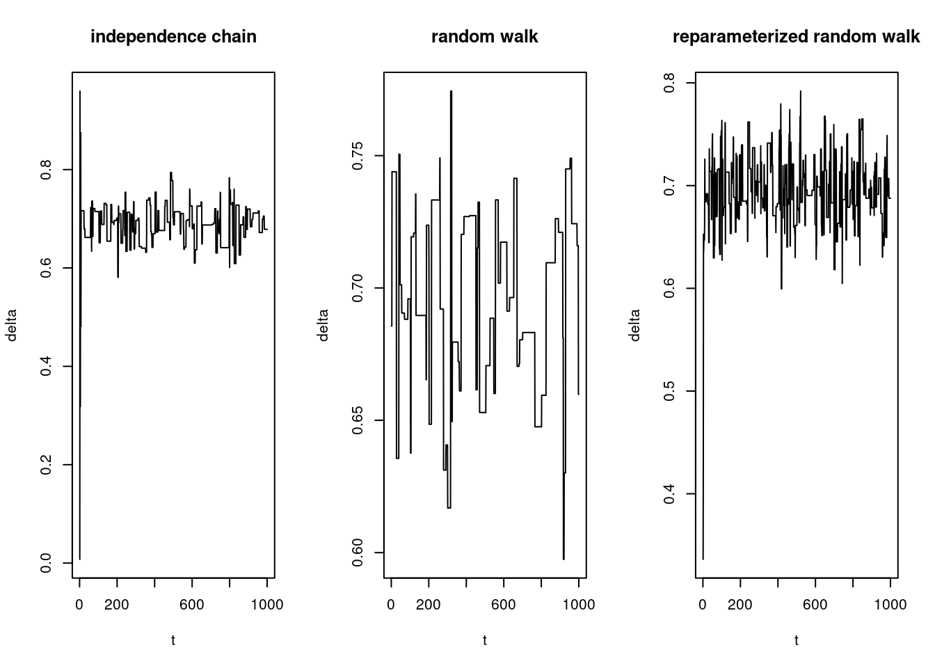

We see that the random walk demonstrates relatively poor mixing. It has a high rejection rate (stays at the same level for long periods of time), causing it to explore the support of the likelihood slowly.

The sample path of the indepedence chain also can be said to demonstrate poor mixing.

The reparameterized random walk exihibits good mixing, vigorously jiggling around the true value.

We plot the ACFs with:

par(mfrow = c(1, 3))
acf(deltas.ic, main = "independence chain")
acf(deltas.rw, main = "random walk")
acf(deltas.u.rw, main = "reparameterized random walk")

They all decay quickly, but in order of increasing autocorrelation: the reparameterized random walk, the independence chain, and the random walk.

In particular, the reparameterized random walk shows autocorrelation that decays quite rapidly with respect to lag time.

Part (a)

Write out the posterior distribution of $(\mu ,\tau )|\overrightarrow{x}$. You may ignore the normalizing constant.

Note that the posterior distribution is given by $$\pi (\mu ,\tau |\overrightarrow{x})=f(\overrightarrow{x}|\tau ,\mu )f(\tau )f(\mu )/Z$$ where $Z=f(\overrightarrow{x})$ is the normalizing constant. We may rewrite this as $$\pi (\mu ,\tau |\overrightarrow{x})\propto L(\tau ,\mu |\overrightarrow{x})f(\tau )f(\mu ).$$

The likelihood function of $(\mu ,\tau )$ conditioned on the data $\overrightarrow{x}$ is given by the product of the normal density on the sample, $$L(\mu ,\tau |\overrightarrow{x})=\prod _{i=1}^n\frac{1}{\sqrt{2\pi {\sigma }^2}}\exp \{-\frac{1}{2{\sigma }^2}(x_i-\mu {)}^2\}$$ which may be simplified to $$L(\mu ,\tau |\overrightarrow{x})={\left(2\pi {\sigma }^2\right)}^{-n/2}\exp \{-\frac{1}{2{\sigma }^2}\sum _{i=1}^n(x_i-\mu {)}^2\}.$$ Observing $\tau =1/{\sigma }^2$, we obtain the result $$L(\mu ,\tau |\overrightarrow{x})\propto {\tau }^{n/2}\exp \{-\frac{\tau }{2}\sum _{i=1}^n(x_i-\mu {)}^2\}.$$ The prior for $\mu$ is $f(\mu )\propto \exp (-\frac{p}{2}(\mu -m{)}^2)$ and the prior for $\tau$ is $f(\tau )\propto {\tau }^{a-1}\exp (-b\tau )$. Putting it all together, we obtain the result $$\pi (\mu ,\tau |\overrightarrow{x})\propto {\tau }^{n/2+a-1}\exp \{-\frac{\tau }{2}\sum _{i=1}^n(x_i-\mu {)}^2-\frac{p}{2}(\mu -m{)}^2-b\tau \}.$$

Part (b)

Show the posterior conditional distribution of $\mu |(\tau ,\overrightarrow{x})$ is $$N(\frac{n\tau \overline{x}+pm}{n\tau +p},\frac{1}{n\tau +p})$$ and the posterior conditional distribution of $\tau |(\mu ,\overrightarrow{x})$ is $$\mathrm{GAM}(a+n/2,b+n/2[s^2+(u-\overline{x}{)}^2]).$$ —

Part (c)

First, generate some ``observed’’ sample data using $x=rnorm(200,mu=5,sigma=2)$. Hand-code Gibbs Sampler algorithm to sample $(\mu ,\tau )$ from the posterior using $x$. You make take prior parameters $a=0.0001;b=0.0001;p=0.0001;m=0$. Use the estimated posterior mean and compare your estimates with the true parameters $\mu =5$ and $\tau =0.25$.

We generate the sample with:

x <- rnorm(200, mean = 5, sd = 2)

We implement the Gibbs sampling with the function:

mu.tau.gibbs <- function(n, x, burn = 1000, theta0 = NULL, p = 1e-04, m = 0, a = 1e-04,
    b = 1e-04) {
    x.mu <- mean(x)
    x.s2 <- var(x)
    x.n <- length(x)

    rmu <- function(tau) {
        mean <- (x.n * tau * x.mu + p * m)/(x.n * tau + p)
        var <- 1/(x.n * tau + p)
        rnorm(1, mean = mean, sd = sqrt(var))
    }

    rtau <- function(mu) {
        rgamma(1, shape = a + x.n/2, rate = b + x.n * (x.s2 + (mu - x.mu)^2)/2)
    }

    prior <- function() {
        c(rnorm(1, m, 1/p), rgamma(1, a, b))
    }

    N <- n + burn
    thetas <- matrix(nrow = N, ncol = 2)
    if (is.null(theta0)) {
        thetas[1, ] <- prior()
    } else {
        thetas[1, ] <- theta0
    }

    for (i in 1:(N - 1)) {
        tau.new <- rtau(thetas[i, 1])
        mu.new <- rmu(tau.new)
        thetas[i + 1, ] <- c(mu.new, tau.new)
    }

    thetas <- thetas[(burn + 1):N, ]
    mu.est <- mean(thetas[, 1])
    tau.est <- mean(thetas[, 2])
    sigma.est <- sqrt(1/tau.est)
    list(theta.dist = thetas, mu.est = mu.est, tau.est = tau.est, sigma.est = sigma.est)
}

We use the Gibbs sampler to estimate $(\mu ,\tau )$ with:

# set up hyper-parameters
a <- 1e-04
b <- 1e-04
m <- 0
p <- 1e-04

res <- mu.tau.gibbs(1e+05, x, burn = 10000, p = p, a = a, m = m, b = b)
mu.est <- round(as.numeric(res$mu.est), digits = 4)
tau.est <- round(as.numeric(res$tau.est), digits = 4)
var.est <- round(1/tau.est, digits = 4)
c(mu.est, tau.est)

## [1] 4.8905 0.2633

We estimate $(\mu ,\tau )$ to be $(4.8905,0.2633{)}^{\prime }$. Therefore, we estimate that the data is being sampled from the normal distribution $$X_i\sim N(\mu =4.8905,{\sigma }^2=3.7979).$$

Additional analysis

Out of curiosity, we decided to plot the marginals of the sample superimposed with their respective conditional densities with:

x.mu <- mean(x)
x.n <- length(x)
x.s2 <- var(x)
mu.dist <- res$theta.dist[, 1]
tau.dist <- res$theta.dist[, 2]

hist(mu.dist, freq = F, breaks = 50, main = "marginal of mu", xlab = "mu")
lines(seq(4, 6, by = 0.01), dnorm(seq(4, 6, by = 0.01), mean = (x.n * tau.est * x.mu)/(x.n *
    tau.est + p), sd = sqrt(1/(x.n * tau.est + p))))

hist(tau.dist, freq = F, breaks = 50, main = "marginal of tau", xlab = "tau")
lines(seq(0.15, 0.4, by = 0.01), dgamma(seq(0.15, 0.4, by = 0.01), shape = a + x.n/2,
    rate = b + x.n * (x.s2 + (mu.est - x.mu)^2)/2))