Part (a)

Write the model for this mixed effects design, defining the fixed effect parameters, and the random effect parameters.

The mixed-effects model is given by \[ Y_{i j k} = \mu + \tau_i + \beta_j + (\tau\!\beta)_{i j} + \epsilon_{i j k} \; \begin{cases} i = 1,\ldots,a=2\\ j = 1,\ldots,b=10\\ k = 1,\ldots,n=3 \end{cases} \] where the fixed effect parameters are \[ \tau_1,\ldots,\tau_a \qquad \left(\sum \tau_i = 0\right) \] and the random effect parameters are \[ \sigma_\beta^2, \sigma_{\tau\!\beta}^2, \sigma^2. \]

Part (b)

Create an interaction plot to display the device effect on hardness measurement.

First, we load the data:

library("readxl")
data = read_excel("handout8data.xlsx")
A = as.factor(na.omit(data$device))
B = as.factor(na.omit(data$specimen))
y = na.omit(data$hardness)

a = length(levels(A))
b = length(levels(B))
N = length(y)
n = N / (a * b)

df.A = a-1
df.B = b-1
df.AB = (a-1)*(b-1)
c("a"=a,"b"=b,"n"=n,"N"=N,"df.A"=df.A,"df.B"=df.B,"df.AB"=df.AB)

##     a     b     n     N  df.A  df.B df.AB 
##     2    10     3    60     1     9     9

The interaction plot is given by:

# remember that we are testing whether operator differences are
# generalizable to a larger population of parts.
interaction.plot(B,A,y)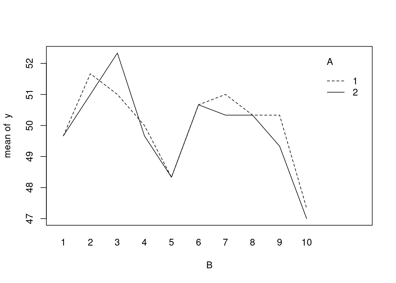

Part (c)

Use a mixed model likelihood approach to test for a systematic difference in the measurements of the two devices. Compute the \(F_0\) statistic, and the \(p\)-value. Provide an interpretation, stated in the context of the problem.

We compute the statistic with:

library("lme4")

## Loading required package: Matrix

contrasts(A)=contr.sum
mixed.mod = lmer(y ~ A + (1|B) + (1|A:B))

## boundary (singular) fit: see help('isSingular')

anova(mixed.mod)

## Analysis of Variance Table
##   npar  Sum Sq Mean Sq F value
## A    1 0.41667 0.41667  0.3121

We see that \(F_0 = .312\) (\(p = .579\)).

Part (d)

Compute estimates of the fixed effect parameters.

The formula for the estimates of the fixed effect parameters \(\{\tau_i\}\) are given by \[ \hat{\tau}_i = \bar{y}_{i \cdot\cdot} - \bar{y}_{\cdot\cdot\cdot} \] for \(i=1,\ldots,a=2\). We use the following R code to compute \(\hat{\tau}_1\):

coef(summary(mixed.mod))

##                Estimate Std. Error     t value
## (Intercept) 49.95000000  0.4282105 116.6482481
## A1           0.08333333  0.1491662   0.5586608

Since \(\tau_1 + \tau_2 = 0\), this means \(\hat{\tau}_1 = .083\) and \(\hat{\tau}_2 = -\hat{\tau}_1 = -.083\).

Part (e)

Now write an \(F_A\) statistic as a ratio of mean squares.

We use Dr. Neath’s custom function \[ \operatorname{mixed.test} : [\text{fixed factors}] \times [\text{random factors}] \times [\text{responses}] \mapsto [\text{statistics}] \] to compute the \(F_A\) statistic:

mixed.test(A,B,y)

##                         SS df         MS
## Fixed Effect A   0.4166667  1  0.4166667
## Random Effect B 99.0166667  9 11.0018519
## Interaction AB   5.4166667  9  0.6018519
## Error           60.0000000 40  1.5000000
##  F-test for fixed effect   p-value
##                0.6923077 0.4269057
##  error.var interaction.var block.var
##        1.5      -0.2993827  1.733333

The \(F\)-test statistic for the factor \(A\) effect is given by \[ F_A = \frac{\operatorname{MS_{A}}}{\operatorname{MS_{A B}}} = .692, \] which has the reference distribution \[ F(\rm{df}_A=a-1,\rm{df}_{A B} = (a-1)(b-1)) = F(1,9). \] Thus, the \(p\)-value is given by \(\Pr\{F(1,9) > F_A\} = .427\).

Part (f)

Write the algebraic formula for the \(F_0\) statistic from a block design on the sample means.

\[ F_0 = \frac {b \sum_{i=1}^{a}(\bar{Y}_{i\cdot\cdot} - \bar{Y}_{\cdot\cdot\cdot})^2/(a-1)} {\sum_{i=1}^{a}\sum_{j=1}^{b}( \bar{Y}_{i j\cdot}- \bar{Y_{i \cdot\cdot}}- \bar{Y}_{\cdot j \cdot}+ \bar{Y}_{\cdot\cdot\cdot} )^2 / (a-1)(b-1)}. \]

Part (g)

Show computationally that (e) and (f) lead to the same test statistic.

We must use the means of the response over repeated measurements of the block (specimen) at a given factor level \(A\). These values have already been computed for us handout8data.xlsx:

# the variables below represent the same data, only with repeat measurements
# summarized by their sample mean.
d = as.factor(na.omit(data$d))
s = as.factor(na.omit(data$s))
h.means = na.omit(data$h)

Now, we do the calculations:

# below we run a randomized block design with the sample means as the
# response variables.
# note that the test for a fixed factor effect is equivalent to that
# from the mixed.test function.
rcbd.mod = lmer(h.means ~ d + (1|s))
anova(rcbd.mod)

## Analysis of Variance Table
##   npar  Sum Sq Mean Sq F value
## d    1 0.13945 0.13945  0.6954

We see that this result matches the result in (e), i.e., mix.test(A,B,y) produced the same result.

Part (h)

Use the result from (g) to argue why interaction mean squares is the appropriate error term.

Repeat measurements are summarized by a sample mean. The test statistic for a block design then leads to the interaction mean squares under a mixed model as the error term.

Part (a)

State the expected value for each of the mean squares.

\[\begin{align*} E(\operatorname{MS_{A}}) &= \sigma^2 + n \sigma_{\tau \! \beta}^2 + \frac{b n \sum_{i=1}^{a}\tau_i^2}{a-1},\\ E(\operatorname{MS_{B}}) &= \sigma^2 + n \sigma_{\tau \! \beta}^2 + a n \sigma_{\beta}^2,\\ E(\operatorname{MS_{A B}}) &= \sigma^2 + n \sigma_{\tau \! \beta}^2,\\ E(\operatorname{MS_{E}}) &= \sigma^2. \end{align*}\]

Part (b)

Compute unbiased estimates for the random effect parameters.

A = as.factor(na.omit(data$op))
B = as.factor(na.omit(data$mach))
y = na.omit(data$strength)
mixed.test(A,B,y)

##                        SS df        MS
## Fixed Effect A  160.33333  2 80.166667
## Random Effect B  12.45833  3  4.152778
## Interaction AB   44.66667  6  7.444444
## Error            45.50000 12  3.791667
##  F-test for fixed effect    p-value
##                 10.76866 0.01034401
##  error.var interaction.var  block.var
##   3.791667        1.826389 -0.5486111

The random effect parameters are given by \(\sigma^2\), \(\sigma_\beta^2\), and \(\sigma_{\tau\beta}^2\). Estimators for these parameters are given by \[\begin{align*} \hat\sigma^2 &= \operatorname{MS_{E}} = 3.792,\\ \hat\sigma_{\beta}^2 &= \frac{\operatorname{MS_{B}}-\operatorname{MS_{A B}}}{a n} = -0.549,\\ \hat\sigma_{\tau\!\beta}^2 &= \frac{\operatorname{MS_{A B}}-\operatorname{MS_{E}}}{n} = 1.826. \end{align*}\]

Part (c)

Use the result from (a) to argue why interaction mean squares is the appropriate error term.

Under the null hypothesis \[ H_0 : \tau_1 = \cdots = \tau_a = 0, \] \(E(\operatorname{MS_{A}}) = \sigma^2 + n \sigma_{\tau \! \beta}^2 + \frac{b n \sum_{i=1}^{a}\tau_i^2}{a-1} = \sigma^2 + n \sigma_{\tau\!\beta}^2\). The scaling requires a denominator with the same expected value. Thus, \(\operatorname{MS_{A B}}\) is the appropriate error term.

Part (d)

Perform a test for operator effects. Compute the \(F_A\) statistic, and the \(p\)-value. Provide an interpretation, stated in the context of the problem.

From part (b), \(F_A = \frac{\operatorname{MS_{A}}}{\operatorname{MS_{A B}}} = 10.769\), which has a \(p\)-value of \(.010\).

Part (e)

Now, use the idea of random factors as an experimental unit to explain why interaction mean squares is the appropriate error term. In particular, comment on how taking repeat measurements on a selected level of a random factor does not increase the pertinent sample size.

Taking repeat measurements at each randomly selected level may serve to increase the measurement accuracy, but does not increase the pertinent sample size. (However, taking repeat measurements does allow us to learn more about the treatment effect at those selected levels, e.g., a therapy may work well for you but is not effective on average.)