Solution: Newton’s method

If we have some function \(f : \mathbb{R} \mapsto \mathbb{R}\) and we wish to find a root of \(f\), i.e., an \(x\) such that \(f(x) = 0\), we may use Newton’s method.

We take an initial guess of the root as \(x_0\) and try to refine it with a linear approximation of \(f\) given by \[ L(f | x_0) = \lambda x.f(x_0) + f'(x_0)(x-x_0). \]

Now, we may approximate a root of \(f\) with a root of \(L(f|x_0)\), \[ L(f|x_0)(x) = 0, \] which may be rewritten as \[ f(x_0) + f'(x_0)(x-x_0) = 0. \] Solving for a root \(x\) of \(L(f|x_0)\) we get the result \[ x = x_0 - \frac{f(x_0)}{f'(x_0)}. \]

Hoping that \(x\) results in a better approximation of the root of \(f\) than \(x_0\), we approximate \(f\) with \(L(f|x)\) and repeat the process.

Generalizing this result, we obtain the iterative procedure \[ x_{i+1} = x_i - \frac{f(x_i)}{f'(x_i)}. \] We continue this process until we obtain some stopping condition, e.g., \(|x_{i+1} - x_i| < \epsilon\).

Letting \(f(x) = x^3 + x - 4\) and \(f'(x) = 3x^2 + 1\) and substituting into the above result, we get the result \[ x_{i+1} = x_i - \frac{x_i^3+x_i-4}{3x_i^2+1}. \]

We implement a general procedure for Newton’s method:

newton_method <- function(f,dfdx,x0,eps,debug=T)
{
  n <- 0
  repeat
  {
    x1 <- x0 - f(x0) / dfdx(x0)
    n <- n + 1
   
    if (debug==T) { cat("iteration=",n," x=",x1,"\n") }
    if(abs(x1 - x0) < eps)
    {
      break
    }
    x0 <- x1
  }
  
  list(root=x0,iter=n)
}

We take an initial guess of \(x_0 = 1\) and \(\epsilon = 1 \times 10^{-6}\) and run the following R code to solve for a root of \(f\) using Newton’s method:

f <- function(x) { x^3 + x - 4 }
dfdx <- function(x) { 3*x^2 + 1 }
eps <- 1e-6
x0 <- 1
result <- newton_method(f,dfdx,x0,eps)

## iteration= 1  x= 1.5 
## iteration= 2  x= 1.387097 
## iteration= 3  x= 1.378839 
## iteration= 4  x= 1.378797 
## iteration= 5  x= 1.378797

We obtain \(x \approx 1.3787967\) after \(5\) iterations. When we plug that approximate root into \(f\) we obtain the result \(f(1.3787967) = 7.3825959\times 10^{-9}\), which is approximately zero.

Solution: Secant method

In Newton’s method, we linearize \(f\) using the derivative of \(f\). If, instead, we use the secant of \(f\) with respect to two inputs \(x_i\) and \(x_{i+1}\), as given by \[ \frac{f(x_{i+1}) - f(x_i)}{x_{i+1}-x_i}, \] we get the iterative procedure \[ x_{i+2} = x_{i+1} - f(x_{i+1})\frac{x_{i+1}-x_i}{f(x_{i+1}) - f(x_i)}, \] which requires two initial values \(x_0\) and \(x_1\).

We define the secant method as a function given by:

secant_method <- function(f,x0,x1,eps,debug=T)
{
  n <- 0
  repeat
  {
    x2 <- x1 - f(x1) * (x1 - x0) / (f(x1) - f(x0))
    n <- n + 1
    
    if (debug==T) { cat("iteration=",n," x=",x2,"\n") }
    
    if(abs(x2-x1) < eps)
    {
      break
    }
    x0 <- x1
    x1 <- x2
  }
  
  list(root=x1,iter=n)
}

We let \(x_0 = 0\), \(x_1 = 1\), and keep everything else the same and run the secant method with the following R code:

x0 <- 0
x1 <- 1
result <- secant_method(f,x0,x1,eps,F)

We obtain \(x \approx 1.3787965\) after \(7\) iterations. When we plug that approximate root into \(f\) we obtain the result \(f(1.3787965) = -1.268648\times 10^{-6}\), which is approximately zero.

Note that this is \(2\) more iterations than Newton’s method.

Comparison of Newton’s method versus secant method

We perform \(10000\) trials to get a better view of how the two methods, Newton and secant, compare over many different initial guesses.

We generate the data with:

n <- 10000
from <- 0
to <- 4
by <- (to-from)/n
newt_sols <- vector(length=n)
sec_sols <- vector(length=n)
i <- 1
for (x0 in seq(from=from, to=to, by=by))
{
  newt_sols[i] <- newton_method(f,dfdx,x0,eps,F)$iter
  sec_sols[i] <- secant_method(f,x0,x0+1,eps,F)$iter
  i <- i + 1
}

We summarize the results and report them with:

cat("mean iterations\n",
    "newton => ", mean(newt_sols), "\n",
    "secant => ", mean(sec_sols), "\n")

## mean iterations
##  newton =>  5.819618 
##  secant =>  7.231077

We see that Newton’s method, on average, requires \(1.4114589\) fewer iterations before the stopping condition is satisfied.

Solution

We are given the following data:

d <- read.table("ache.txt", header=T)
n <- length(d$age)
X <- cbind(rep(1,n), d$age, d$age^2)

loglike <- function(theta)
{
  sum(dpois(d$monkeys,exp(log(d$days)+X%*%theta),log=T))
}

We generalize the univariate Newton’s method in Problem 1 to the multivariate case. We implement the multivariate Newton-Raphson method with numerical hessian and jacobian with the following R code:

library(numDeriv)
newton_raphson_method <- function(x0,f,eps)
{
  n <- 0
  x1 <- x0
  repeat
  {
      x1 <- x0 - solve(hessian(f,x0))%*%t(jacobian(f,x0))
      n <- n + 1
      if (n %% 7 == 0) { cat("iteration=",n," theta=",x1,"\n") }
      if (max(abs(x1 - x0)) < eps)
      {
        break
      }
      x0 <- x1
  }
  list(root=x1,iter=n)
}

We use the multivariate Newton-Raphson method to find the MLE of \(\theta\) in the poisson regression model:

eps <- 1e-6
theta0 <- c(5.99, 0.167, 0.001) # starting values
theta_mle <- newton_raphson_method(theta0,loglike,eps)$root

## iteration= 7  theta= -1.01133 0.1670442 0.0009996348 
## iteration= 14  theta= -7.590958 0.1532685 0.001112005 
## iteration= 21  theta= 1.438482 -0.2696711 0.003827083 
## iteration= 28  theta= -5.484246 0.1246477 -0.001203418

The MLE of \(\theta\) is given by:

theta_mle

##              [,1]
## [1,] -5.484245904
## [2,]  0.124647667
## [3,] -0.001203418

We compare the results with the builtin method:

glm(monkeys~age+I(age^2),family="poisson", offset=log(days),data=d)$coefficients

##  (Intercept)          age     I(age^2) 
## -5.484245904  0.124647667 -0.001203418

The hand-coded approach and the builtin approach obtain the same point estimate \(\hat\theta = (-5.4842, 0.1246, -0.0012)'\).

Solution: part (a)

Standard logistic distribution \[ F(x) = \frac{1}{1+e^{-x}} \]

Solve for \(x\) in \[\begin{align*} u &= F(x)\\ u &= \frac{1}{1+e^{-x}}\\ x &= \log(u/(1-u)). \end{align*}\]

n <- 10000
us <- runif(n)
d1 <- density(log(us/(1-us)))
d2 <- density(rlogis(n))
plot(d1,col="blue",main="comparison of density plots")
lines(d2,col="red")
legend(x="topright",legend=c("inverse method","built-in"),col=c("blue","red"),
       pch=c("-","-"))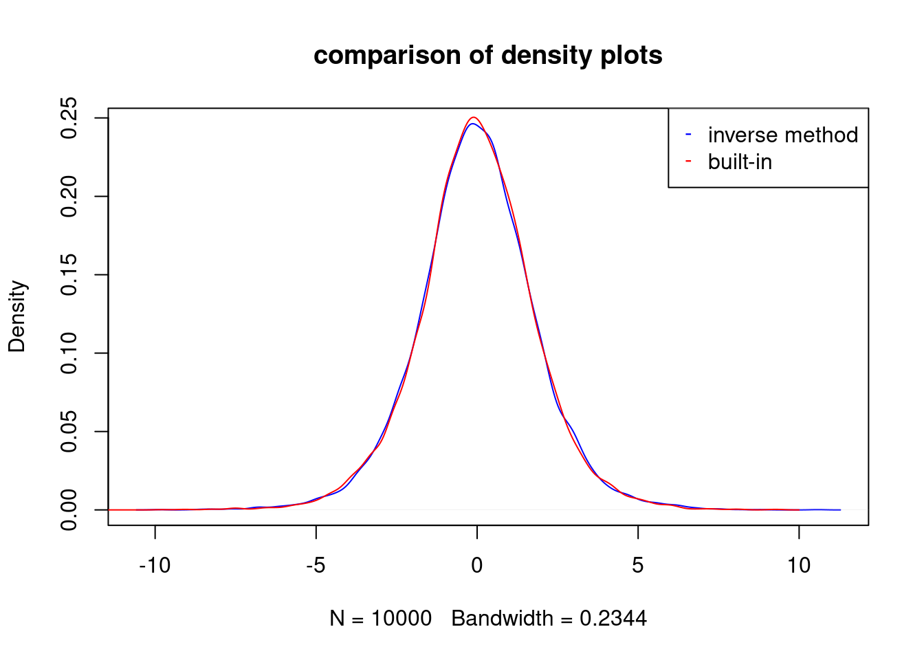

Solution: part (b)

Standard Cauchy distribution \[ F(x) = \frac{1}{2} + \frac{1}{\pi} \operatorname{arctan(x)} \]

Solve for \(x\) in \[\begin{align*} u &= F(x)\\ u &= \frac{1}{2} + \frac{1}{\pi} \operatorname{arctan(x)}\\ x &= \tan(\pi(u-1/2)). \end{align*}\]

n <- 1000
us <- runif(n)
d1 <- tan(pi*(us-0.5))
d2 <- rcauchy(n=n)

d1 <- d1[d1 > -20 & d1 < 20]
d2 <- d2[d2 > -20 & d2 < 20]

c1 <- rgb(0,0,255, max = 255, alpha = 50, names = "blue")
c2 <- rgb(255,0,0, max = 255, alpha = 50, names = "red")

par(mfrow=c(1,2))
hist(d1,col=c1,freq=F,breaks=50,main="inverse-transform method vs built-in")
hist(d2,col=c2,add=T,freq=F,breaks=50)
legend(x="topright",legend=c("inv","builtin"),col=c("blue","red"),pch=c("-","-"))
plot(density(d1), col="blue",main="density plot")
lines(density(d2), col="red") 
legend(x="topright",legend=c("inv","builtin"),col=c("blue","red"),pch=c("-","-"))

Solution

A random variable \(X \sim \operatorname{Geometric(p)}\) is given by the number of i.i.d. trials needed to have a success where success occurs with probability \(p\).

Thus, we may simulate this distribution with the following R code:

# simulate n realizes of geometric(p)
rgeo <- function(n,p)
{
  outcomes <- vector(length=n)
  for (i in 1:n)
  {
    trials <- 0
    while (T)
    {
      trials <- trials + 1
      if (rbinom(1,1,p) == 1)
      {
        break
      }
    }
    outcomes[i] <- trials
  }
  outcomes
}

When we use this function to draw a sample of \(n=10000\) geoemtrically distributed random variables with \(p=0.2\), we obtain:

p <- .2
n <- 10000
sample <- rgeo(n,p)
cat("the mean should be approximate 1/p =", 1/p, " and we obtain a mean of ", mean(sample))

## the mean should be approximate 1/p = 5  and we obtain a mean of  5.0425

Solution

We are given the density of the standard half-normal distribution, \[ \operatorname{dhalfnormal}(x) = \frac{2}{\sqrt{2 \pi}} e^{-x^2/2}, x > 0. \]

We model this density with the following R code:

# density for standard half-normal
dhalfnormal <- function(x) { 2/sqrt(2*pi)*exp(-x^2/2) }

We sample from the exponential distribution \(\operatorname{EXP}(\lambda=1)\), with density \(g\) and thus we first find the \(c\) satisfying \[ c = \max \left\{ \frac{\operatorname{dhalfnormal}(x)}{\operatorname{dexp}(x|\lambda=1)} | x \in \mathbb{R} \right\}, \] which is found to be approximately \(c = 1.315489247\).

We implement the standard half-normal sampler, \(\operatorname{rhalfnormal}\), using the acceptance-rejection sampling technique with the following R code:

# accept-rejection sampling for standard half-normal
# using exp(rate=1)
rhalfnormal <- function(N)
{
  c <- 1.315489247
  xs <- vector(length=N)
  k <- 1
  while (T)
  {
    x <- rexp(n=1)
    if (runif(n=1) < dhalfnormal(x)/(c*dexp(x)))
    {
      xs[k] <- x
      k <- k + 1
      if (k == N)
      {
        break
      }
    }
  }
  xs
}

We simulate drawing \(n=100000\) samples from the standard half-normal distribution and plotting a histogram of the sample with its density overload in red on top of it with the following R code:

n <- 100000
sample <- rhalfnormal(n)
hist(sample,freq=F,breaks=50,main="standard half-normal")
curve(dhalfnormal(x),add=TRUE,col="red")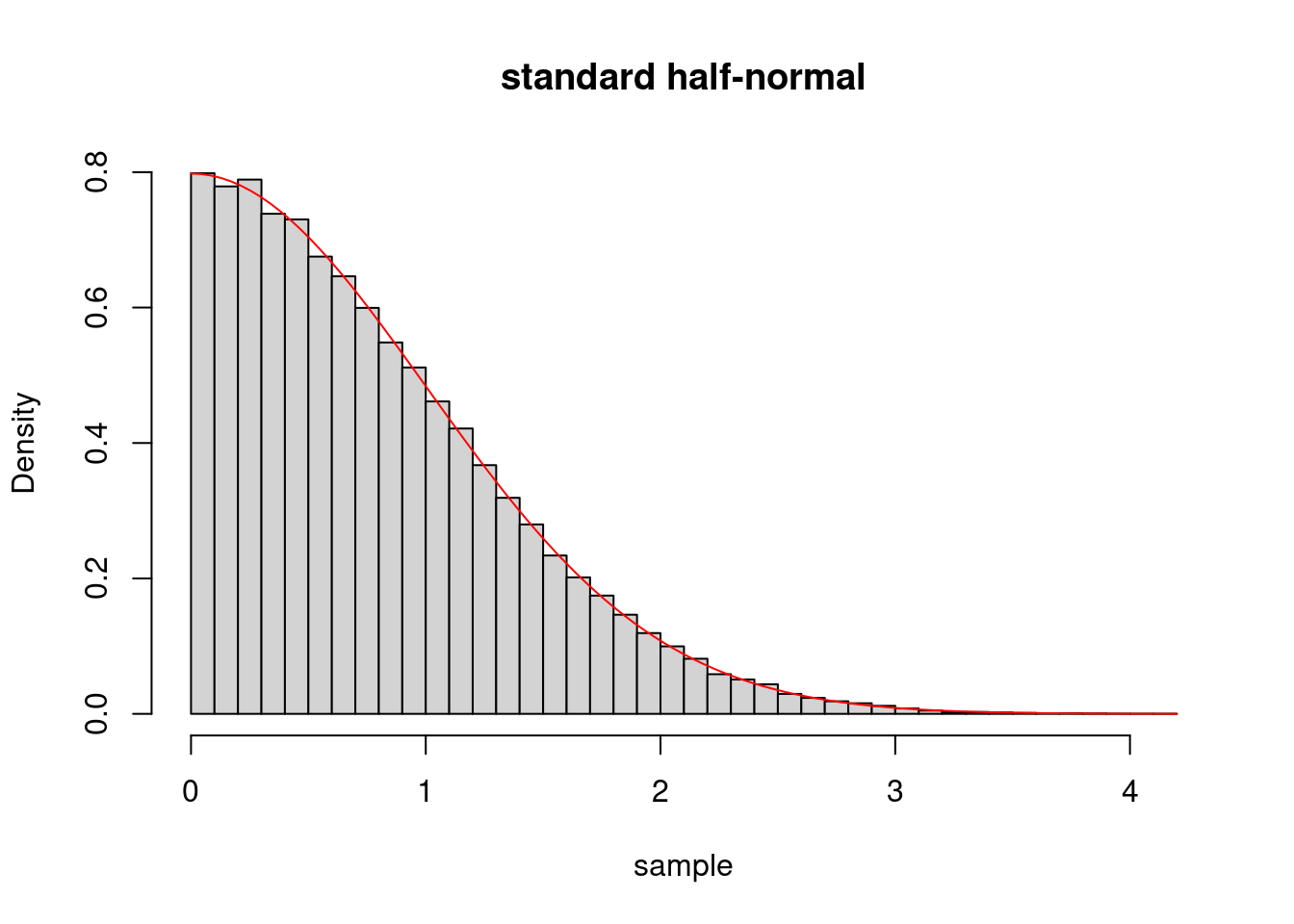 

We see that the histogram is compatible with being drawn from the overload density.

Solution

We are given the kernel of the bimodal distribution of interest, \[ \operatorname{ker-bimodal}(x) = 3 e^{-0.5(x+2)^2} + 7 e^{-0.5(x-2)^2}, \] with the normalizing constant \(C = 25.0663\) and thus the pdf for the bimodal is given by \[ \operatorname{dbimodal}(x) = \frac{\operatorname{ker}(x)}{C}. \]

We model these two functions with the following R code:

# density for biomodal density
kerbimodal <- function(x) { 3*exp(-0.5*(x+2)^2) + 7*exp(-0.5*(x-2)^2) }
kerbimodal.C <- 25.0663
dbimodal <- function(x) { kerbimodal(x) / kerbimodal.C }

We sample from the normal distribution \(N(\mu=0,\sigma^2=2^2)\), with density \(g\) and thus we first find the \(c\) satisfying \[ c = \max \left\{ \frac{\operatorname{ker-bimodal}(x)}{g(x|\mu=0,\sigma^2=2^2)} | x \in \mathbb{R} \right\}, \] which is found to be approximately \(c = 68.35212\).

We implement the bimodal sampler, \(\operatorname{rbimodal}\), using the acceptance-rejection sampling technique with the following R code:

# accept-rejection sampling for bimodal distribution with density dbimodal
# using normal(0,2^2).
rbimodal <- function(N)
{
  c <- 68.35212
  xs <- vector(length=N)
  k <- 1
  while (T)
  {
    x <- rnorm(n=1,mean=0,sd=2)
    if (runif(n=1) < kerbimodal(x)/(c*dnorm(x,mean=0,sd=2)))
    {
      xs[k] <- x
      if (k == N)
      {
        break
      }
      k <- k + 1
    }
  }
  xs
}

We simulate drawing \(n=100000\) samples from the bimodal distribution and plotting a histogram of the sample with its density overload in red on top of it with the following R code:

n <- 100000
sample <- rbimodal(n)
hist(sample,freq=F,breaks=50,main="bimodal")
curve(dbimodal(x),add=TRUE,col="red") 

We see that the histogram is compatible with being drawn from the overload density.