Last post was the bad news: a real qubit leaks its coherence into the environment and forgets what it was doing. This post is the reason quantum computing is not therefore hopeless. You can detect errors and undo them, even on a state you are forbidden to look at, by spreading one logical qubit across several physical ones. The idea is old (classical codes repeat bits and take a majority vote) but the quantum version has to get past two walls that do not exist classically: you cannot copy an unknown qubit, and looking at a qubit destroys its superposition. The 3-qubit code threads both needles, and building it is a fitting last thing to build.
import numpy as np
import matplotlib.pyplot as plt

from qfs import gates
from qfs.dense import embed
from qfs.qec import (
    encode_bitflip, bitflip_syndrome, correct_bitflip, decode_bitflip,
    run_phaseflip_code,
)
Encoding without cloning
A logical qubit $a|0\rangle + b|1\rangle$ is encoded as $a|000\rangle + b|111\rangle$. This looks like copying, but it is not: there is no operation that copies an unknown qubit, and we are not doing one. We start with the logical qubit on wire 0 and use two CNOTs to entangle wires 1 and 2 with it. The three physical qubits now hold one logical qubit as an inseparable whole, and crucially $a$ and $b$ are never duplicated or read.
a, b = 0.6, 0.8
encoded = encode_bitflip(a, b)
print("encoded amplitudes (only |000> and |111> nonzero):")
print("  |000>:", round(encoded[0b000].real, 3), "   |111>:", round(encoded[0b111].real, 3))
encoded amplitudes (only |000> and |111> nonzero):
  |000>: 0.6    |111>: 0.8
The syndrome: finding the error without reading the data
Now flip one qubit, say qubit 1. The state becomes $a|010\rangle + b|101\rangle$. We need to learn which qubit flipped without learning anything about $a$ and $b$, because measuring $a$ or $b$ would collapse the superposition we are trying to protect. The trick is to measure two parities: $Z_0 Z_1$ asks “do qubits 0 and 1 agree?” and $Z_1 Z_2$ asks the same of 1 and 2. A parity is the same for the $|0\ldots\rangle$ branch and the $|1\ldots\rangle$ branch, so it reveals the error location and nothing about the logical state. The pair of answers is the syndrome. (Our simulator reads the parities as expectation values, which is exact here because a code state with at most one flip is a $\pm 1$ eigenstate of both parities; on hardware the same answers come from ancilla-assisted measurements.)
for error_qubit in (None, 0, 1, 2):
    psi = encode_bitflip(a, b)
    if error_qubit is not None:
        psi = embed(gates.X, error_qubit, 3) @ psi
    print(f"error on qubit {str(error_qubit):4s} -> syndrome {bitflip_syndrome(psi)}")
error on qubit None -> syndrome (1, 1)
error on qubit 0    -> syndrome (-1, 1)
error on qubit 1    -> syndrome (-1, -1)
error on qubit 2    -> syndrome (1, -1)
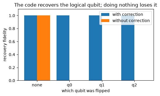
Each error gives a distinct syndrome, so the syndrome tells us exactly which qubit to flip back. Apply the correction, reverse the encoding, and the logical qubit comes out untouched. Here is the whole loop. The fidelity below is strict: it asks whether the full register returns to the original logical state with clean $|00\rangle$ ancillas. With correction it is 1 for any single bit-flip error. Without correction it is 0, though for a different reason at each location: a flip on the logical wire flips the stored qubit itself, while a flip on wire 1 or 2 leaves the logical qubit intact but strands the ancillas dirty, outside the code space.
def fidelity(a, b, error_qubit, correct):
    psi = encode_bitflip(a, b)
    if error_qubit is not None:
        psi = embed(gates.X, error_qubit, 3) @ psi
    if correct:
        psi = correct_bitflip(psi)
    psi = decode_bitflip(psi)
    return abs(np.conj(a) * psi[0] + np.conj(b) * psi[0b100])


labels = ["none", "q0", "q1", "q2"]
errors = [None, 0, 1, 2]
with_corr = [fidelity(a, b, e, True) for e in errors]
without = [fidelity(a, b, e, False) for e in errors]

x = np.arange(len(labels))
fig, ax = plt.subplots(figsize=(6, 3.2))
ax.bar(x - 0.2, with_corr, 0.4, label="with correction")
ax.bar(x + 0.2, without, 0.4, label="without correction")
ax.set_xticks(x); ax.set_xticklabels(labels)
ax.set_ylabel("recovery fidelity"); ax.set_ylim(0, 1.1)
ax.set_xlabel("which qubit was flipped")
ax.set_title("The code recovers the logical qubit; doing nothing loses it")
ax.legend()
plt.show()
Phase errors, and the other code
This code only catches bit flips. A phase error, a $Z$ that sends $|1\rangle$ to $-|1\rangle$, commutes with the $Z$ parities and slips through invisibly. But there is a beautiful fix: a phase error in the computational basis is a bit flip in the Hadamard basis, because $HZH = X$. So sandwich the same machinery between layers of Hadamards and you get a code that corrects $Z$ errors instead. The phase-flip code recovers the logical state under any single $Z$ error.
a, b = 0.6, 0.8
for error_qubit in (0, 1, 2):
    ra, rb = run_phaseflip_code(a, b, error_qubit=error_qubit)
    print(f"phase error on qubit {error_qubit} -> recovered ({round(ra.real,3)}, {round(rb.real,3)})  (input was {a}, {b})")
phase error on qubit 0 -> recovered (0.6, 0.8)  (input was 0.6, 0.8)
phase error on qubit 1 -> recovered (0.6, 0.8)  (input was 0.6, 0.8)
phase error on qubit 2 -> recovered (0.6, 0.8)  (input was 0.6, 0.8)
The full Shor 9-qubit code stacks these two ideas, three blocks of the phase-flip code each protected by the bit-flip code, to correct an arbitrary single-qubit error (any combination of $X$ and $Z$, including $Y$). It is the same construction twice, and we will leave it as the natural next exercise.
The honest limit, and the way past it
This is a distance-3 code: it corrects one error and fails on two. Two flips produce a syndrome that points at the innocent third qubit, the correction makes things worse, and the logical qubit flips. There is no magic here, just a code too small to tell one story from another.
psi = encode_bitflip(1, 0)                              # logical |0>
psi = embed(gates.X, 0, 3) @ embed(gates.X, 1, 3) @ psi  # two flips
out = decode_bitflip(correct_bitflip(psi))
print("two errors: logical |0> was miscorrected into |1>:", np.allclose([out[0], out[0b100]], [0, 1]))
two errors: logical |0> was miscorrected into |1>: True
The arithmetic that rescues this: if each physical qubit flips independently with probability $p$, the encoded qubit fails only when two or three flips land, with probability $3p^2(1-p) + p^3$. That beats the bare qubit’s $p$ exactly when $p < 1/2$. Encoding wins whenever the hardware is already better than a coin flip, and the margin widens as $p$ shrinks.
Real machines use bigger codes, the surface code chief among them, that correct more errors by using many more physical qubits per logical one. The deep result that makes the whole enterprise possible is the threshold theorem: if the physical error rate is below a fixed threshold, you can drive the logical error rate as low as you like by scaling the code up, faster than the errors accumulate. Below the threshold, a noisy machine can compute reliably forever. That is the promise the entire field is built on.
The end of the book
We started, ten posts ago, with the claim that a qubit is just a unit vector in $\mathbb{C}^2$ and that everything mysterious about quantum computing is something you can watch happen inside an array. We have now cashed that claim in full. Superposition and interference were complex numbers adding and cancelling. Entanglement was a vector that would not factor. Measurement was sampling and renormalizing. The famous algorithms (Deutsch-Jozsa, Grover, the Fourier transform, phase estimation, Shor’s factoring) were each a few lines of NumPy, with the Fourier transform and the circuit engine checked against Qiskit directly. Then mixed states, noise, decoherence, and finally error correction showed us the real machine, the one that leaks and the one engineers fight to protect.
The whole simulator is about three hundred lines of Python and a hundred and fifty tests. None of it needed a quantum computer, or a framework, or anything beyond a length-two complex array and the patience to follow the linear algebra wherever it went. That was always the point. The spooky parts are not spooky once you build them. They are just what the math does.
Watch the Episode
This post is also a video episode: Noise, Decoherence, and Why Error Correction Is Hard, part of the series playlist.
Discussion