Last post ended with a warning: the off-diagonal coherences of a density matrix are the fragile part, and a real qubit loses them on its own. This post makes that concrete. A real qubit is never isolated. It is weakly, continuously entangling itself with its environment, the stray fields and vibrations and photons around it, and the environment is precisely the thing we have no choice but to trace away. Post 8 showed that tracing away an entangled partner turns a pure state mixed. Do it continuously and the qubit decays. We package that decay as a channel: a set of Kraus operators that evolve the density matrix as $\rho \mapsto \sum_k K_k, \rho, K_k^\dagger$, the non-unitary cousin of a gate.
import numpy as np
import matplotlib.pyplot as plt

from qfs import gates
from qfs.density import DensityMatrix
from qfs.channels import amplitude_damping, phase_damping, depolarizing, apply_channel
Two ways to decay
Hardware people measure two times, called T1 and T2, and they correspond to two channels. Amplitude damping is energy loss: an excited $|1\rangle$ relaxes to $|0\rangle$ with some probability. Start a qubit in $|1\rangle$ and its excited population bleeds away.
dm = DensityMatrix.from_statevector([0, 1])     # |1>
for _ in range(3):
    apply_channel(dm, amplitude_damping(0.3), 0)
print("P(excited) after 3 rounds of amplitude damping:", round(dm.probabilities()[1], 3))
P(excited) after 3 rounds of amplitude damping: 0.343
Phase damping is subtler and, for quantum computing, deadlier. It takes no energy, the populations on the diagonal never move, but it shrinks the off-diagonal coherence. The qubit keeps its probabilities and loses its quantum-ness. Put a qubit in $|+\rangle$, where the coherence is maximal, and watch only the off-diagonal fall.
dm = DensityMatrix(1).apply(gates.H, 0)         # |+>: coherence 0.5
print("before: populations", dm.probabilities(), " coherence", round(abs(dm.rho[0, 1]), 3))
apply_channel(dm, phase_damping(0.5), 0)
print("after:  populations", dm.probabilities(), " coherence", round(abs(dm.rho[0, 1]), 3))
before: populations [0.5 0.5]  coherence 0.5
after:  populations [0.5 0.5]  coherence 0.354
Each pass of phase_damping(lam) scales the off-diagonal by $\sqrt{1-\lambda}$,
so one application at $\lambda = 0.5$ takes the coherence from $0.5$ to
$0.5\sqrt{0.5} \approx 0.354$. The populations never move; only the phase
relationship decays.
Watching coherence die
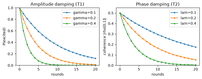
Both processes are exponential. Here they are side by side: amplitude damping draining the excited population (T1), and phase damping draining the coherence (T2), each for a few noise strengths. This is the picture of why a quantum computer has a clock it is racing against.
steps = np.arange(0, 21)
fig, (ax1, ax2) = plt.subplots(1, 2, figsize=(8, 3.2))

for gamma in (0.1, 0.2, 0.4):
    pops = []
    dm = DensityMatrix.from_statevector([0, 1])
    for _ in steps:
        pops.append(dm.probabilities()[1])
        apply_channel(dm, amplitude_damping(gamma), 0)
    ax1.plot(steps, pops, marker="o", markersize=3, label=f"gamma={gamma}")
ax1.set_title("Amplitude damping (T1)")
ax1.set_xlabel("rounds"); ax1.set_ylabel("P(excited)"); ax1.set_ylim(0, 1); ax1.legend()

for lam in (0.1, 0.2, 0.4):
    cohs = []
    dm = DensityMatrix(1).apply(gates.H, 0)
    for _ in steps:
        cohs.append(abs(dm.rho[0, 1]))
        apply_channel(dm, phase_damping(lam), 0)
    ax2.plot(steps, cohs, marker="o", markersize=3, label=f"lam={lam}")
ax2.set_title("Phase damping (T2)")
ax2.set_xlabel("rounds"); ax2.set_ylabel("coherence |rho[0,1]|"); ax2.set_ylim(0, 0.55); ax2.legend()

plt.tight_layout()
plt.show()
Decoherence on an entangled state
The same thing happens to entanglement, which is the resource the algorithms run on. Take a Bell state, whose coherence lives in the corner entries $\rho_{0,3}$ and $\rho_{3,0}$, and dephase one of its two qubits. The shared coherence decays even though we only touched one side, and the once-pure entangled pair drifts toward a boring classical mixture of $|00\rangle$ and $|11\rangle$.
dm = DensityMatrix.from_statevector([1 / np.sqrt(2), 0, 0, 1 / np.sqrt(2)])
print("Bell coherence rho[0,3]:", round(abs(dm.rho[0, 3]), 3))
for _ in range(20):
    apply_channel(dm, phase_damping(0.3), 0)
print("after 20 rounds on one qubit:", round(abs(dm.rho[0, 3]), 4))
print("populations untouched:", np.allclose(np.diag(dm.rho).real, [0.5, 0, 0, 0.5]))
print("purity dropped from 1 toward 1/2:", round(np.trace(dm.rho @ dm.rho).real, 3))
Bell coherence rho[0,3]: 0.5
after 20 rounds on one qubit: 0.0141
populations untouched: True
purity dropped from 1 toward 1/2: 0.5
The whole zoo
Two more channels round out the standard set. Depolarizing is the pessimist’s model: with some probability the qubit is simply replaced by noise, dragging any state toward the maximally mixed $\tfrac{1}{2}I$. Bit flip and phase flip apply an $X$ or a $Z$ with probability $p$; they are the discrete errors a code can catch, and they are exactly what the next post defends against.
dm = DensityMatrix.from_statevector([1, 0])
apply_channel(dm, depolarizing(0.75), 0)
print("depolarizing(0.75) on |0> drifts toward I/2:\n", np.round(dm.rho, 3))
depolarizing(0.75) on |0> drifts toward I/2:
 [[0.625+0.j 0.   +0.j]
 [0.   +0.j 0.375+0.j]]
Where this leaves us
Noise is not a bug in the model, it is the honest consequence of the density matrix meeting the real world. Energy leaks (amplitude damping), phase scrambles (phase damping), and either way the coherences that make a qubit more than a classical bit fade toward zero. That is the central engineering problem of quantum computing, and the reason a circuit has to finish before its qubits forget what they were doing.
We are not, however, helpless. The discrete errors at the end, the stray $X$ and $Z$ flips, can be detected and undone without ever measuring the protected data, by spreading one logical qubit across several physical ones. That is quantum error correction, the last post and the reason a noisy machine can still, in principle, compute forever.
Watch the Episode
This post is also a video episode: Noise, Decoherence, and Why Error Correction Is Hard, part of the series playlist.
Discussion