
Every state in this series so far has been a single vector with definite amplitudes. That picture is not wrong, but it is incomplete, and this post is about the gap. There are two ordinary situations a state vector cannot describe. The first is plain ignorance: someone hands you a qubit that is $|0\rangle$ half the time and $|1\rangle$ the other half, and you do not know which. The second is deeper: take one qubit of an entangled pair and ask what state it is in, on its own. We saw in post 1 that there is no answer. Both situations need a richer object, the density matrix, and the striking thing is that it cannot tell the two situations apart.
import numpy as np
import matplotlib.pyplot as plt

from qfs import gates
from qfs.density import DensityMatrix
The density matrix of a pure state
For a pure state $|\psi\rangle$ the density matrix is just the outer product $\rho = |\psi\rangle\langle\psi|$. It carries the same information as the vector, arranged in a square. The diagonal holds the measurement probabilities; the off-diagonal entries are coherences, the part that records genuine quantum superposition. Here is $|+\rangle = \frac{1}{\sqrt 2}(|0\rangle + |1\rangle)$.
plus = DensityMatrix(1).apply(gates.H, 0)
print("rho for |+>:\n", np.round(plus.rho, 3))
print("diagonal (probabilities):", plus.probabilities())
rho for |+>:
 [[0.5+0.j 0.5+0.j]
 [0.5+0.j 0.5+0.j]]
diagonal (probabilities): [0.5 0.5]
All four entries are $1/2$. The off-diagonal $1/2$ is the coherence between $|0\rangle$ and $|1\rangle$. A useful number is the purity, $\mathrm{Tr}(\rho^2)$: it is exactly $1$ for a pure state and drops below $1$ as the state becomes mixed.
print("purity of |+>:", np.trace(plus.rho @ plus.rho).real)
purity of |+>: 0.9999999999999996
The two faces of a mixed state
Now the two situations. First, classical ignorance: a 50/50 mixture of $|0\rangle$ and $|1\rangle$. You build that density matrix by averaging the two pure ones.
mixture = 0.5 * np.outer([1, 0], [1, 0]) + 0.5 * np.outer([0, 1], [0, 1])
print("50/50 classical mixture:\n", np.round(mixture, 3))
50/50 classical mixture:
 [[0.5 0. ]
 [0.  0.5]]
Second, entanglement. Build a Bell state, which is pure and perfectly definite as a
whole, and then trace out the second qubit to ask about the first one alone.
Tracing out is a sum over the discarded qubit’s matched indices,
$(\rho_A){ij} = \sum_k \rho{ik,jk}$, and partial_trace is exactly that sum.
bell = DensityMatrix.from_statevector([1 / np.sqrt(2), 0, 0, 1 / np.sqrt(2)])
reduced = bell.partial_trace(keep=[0])
print("one qubit of a Bell pair:\n", np.round(reduced.rho, 3))
print("identical to the classical mixture:", np.allclose(reduced.rho, mixture))
one qubit of a Bell pair:
 [[0.5+0.j 0. +0.j]
 [0. +0.j 0.5+0.j]]
identical to the classical mixture: True
They are the same matrix, $\tfrac{1}{2}I$. This is the heart of the subject. The qubit you got by tracing away its entangled partner is, from where you stand, indistinguishable from a coin you flipped and did not look at. Quantum ignorance and classical ignorance arrive at the same object. Both have purity $1/2$, the most mixed a single qubit can be, even though the Bell pair they came from was perfectly pure.
print("purity of the Bell pair (whole):", round(np.trace(bell.rho @ bell.rho).real, 3))
print("purity of one qubit (reduced):  ", round(np.trace(reduced.rho @ reduced.rho).real, 3))
purity of the Bell pair (whole): 1.0
purity of one qubit (reduced):   0.5
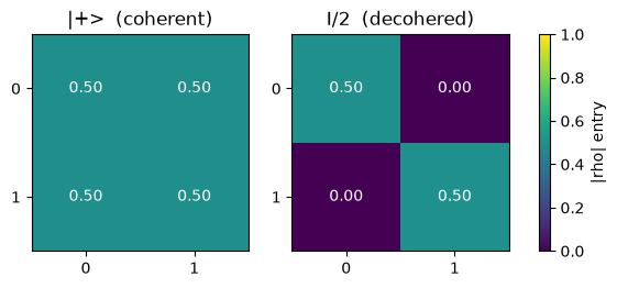
Coherence is the off-diagonal
It pays to look at this. A pure superposition has off-diagonal coherence; a fully mixed state has none, only the diagonal populations survive. The picture on the left is a live superposition, the one on the right is a classical coin. The whole next post is about the arrow between them.
fig, (ax1, ax2) = plt.subplots(1, 2, figsize=(7, 3.2))
for ax, rho, title in [(ax1, plus.rho, "|+>  (coherent)"), (ax2, mixture, "I/2  (decohered)")]:
    im = ax.imshow(np.abs(rho), vmin=0, vmax=1, cmap="viridis")
    ax.set_xticks([0, 1]); ax.set_yticks([0, 1])
    ax.set_xticklabels(["0", "1"]); ax.set_yticklabels(["0", "1"])
    ax.set_title(title)
    for i in range(2):
        for j in range(2):
            ax.text(j, i, f"{abs(rho[i, j]):.2f}", ha="center", va="center", color="white")
fig.colorbar(im, ax=[ax1, ax2], label="|rho| entry", shrink=0.8)
plt.show()
It still does everything the statevector did
The density matrix is a strict generalization, so on pure states it reproduces the old machinery. Gates evolve it as $\rho \mapsto U \rho U^\dagger$, probabilities are the diagonal, and expectation values are $\mathrm{Tr}(O\rho)$. A noiseless circuit on a density matrix tracks $|\psi\rangle\langle\psi|$ exactly, which is the sanity check that we built it right.
dm = DensityMatrix(1).apply(gates.Ry(np.pi / 3), 0)
print("expectation <Z> via Tr(Z rho):", round(dm.expectation(gates.Z), 4))
print("matches cos(pi/3):            ", round(np.cos(np.pi / 3), 4))
expectation <Z> via Tr(Z rho): 0.5
matches cos(pi/3):             0.5
Where this leaves us
The density matrix is the honest description of a quantum state when you are not in possession of the whole story, which, for any real qubit, you never are. Its two sources of mixedness, classical ignorance and traced-away entanglement, are the same object, and its off-diagonal coherences are the fragile part that makes a qubit quantum.
That fragility is the next post. A real qubit is ceaselessly, weakly entangling itself with its environment, and the environment is exactly the thing we trace away. The result is that the off-diagonals we just plotted decay toward zero on their own. That process is decoherence, we model it with noise channels, and it is the reason quantum computers are hard to build.
Watch the Episode
This post is also a video episode: Mixed States and the Density Matrix, part of the series playlist.
Discussion