
This post does not add a quantum idea. It fixes an engineering mistake we have been making since post 1, on purpose, because it was the clearest thing to build first. Every gate so far has been applied by constructing a dense matrix of size 2^n by 2^n and multiplying the statevector by it. That matrix has 4^n entries. A few qubits past a dozen it stops fitting in memory, at fifteen qubits it is already 17 GB, which is why Shor’s algorithm last post handled N = 15 but could not reach N = 21. The fix is to never build the matrix at all.
import time

import numpy as np
import matplotlib.pyplot as plt

from qfs import gates
from qfs.dense import embed
from qfs.tensor import apply_gate
from qfs.statevector import StateVector
A statevector is a tensor
The amplitudes are a flat array of length 2^n, but they are indexed by n bits,
one per qubit. So the natural shape is not a vector, it is an n-dimensional grid
with two entries along each axis: a rank-n tensor, with axis q belonging to
qubit q. Reshaping is free, just a reinterpretation of the same buffer.
n = 3
amps = StateVector(n).apply(gates.H, 0).apply(gates.X, 2, controls=(0,)).amps
print("flat shape: ", amps.shape)
print("tensor shape:", amps.reshape([2] * n).shape)
flat shape:  (8,)
tensor shape: (2, 2, 2)
A k-qubit gate is also a tensor: a 2^k by 2^k matrix is really 2k axes, k
for its inputs and k for its outputs. Applying the gate is a contraction: glue
the gate’s input axes to the state’s target axes, sum over them, and leave every
other qubit’s axis untouched. That is one np.tensordot call, and it costs
O(2^n) instead of O(4^n) because it never visits the qubits the gate does not act
on. The whole engine is six lines.
import inspect
print(inspect.getsource(apply_gate))
def apply_gate(amps, U, targets, n):
    """Apply k-qubit gate U to `targets` of an n-qubit statevector by contraction.

    U is 2^k x 2^k (k = len(targets)). The order of `targets` is part of the
    contract: gate wire i (the i-th pair of row/column indices of U, big-endian)
    acts on qubit targets[i], so targets=[c, t] and targets=[t, c] with the same U
    are different operations. Returns the new length-2^n amplitude vector. Cost is
    O(2^n), versus O(4^n) to build the dense operator.
    """
    k = len(targets)
    psi = amps.reshape([2] * n)
    Ut = U.reshape([2] * (2 * k))
    psi = np.tensordot(Ut, psi, axes=(list(range(k, 2 * k)), list(targets)))
    psi = np.moveaxis(psi, list(range(k)), list(targets))
    return psi.reshape(2 ** n)
It agrees with the dense engine, exactly
This is the same operation we have been doing, computed a cheaper way, so it had better give the same answer. It does, to floating-point precision, for single-qubit gates and for controlled gates alike.
rng = np.random.default_rng(0)
v = rng.normal(size=2 ** 4) + 1j * rng.normal(size=2 ** 4)
v /= np.linalg.norm(v)

same_1q = np.allclose(apply_gate(v, gates.H, [2], 4), embed(gates.H, 2, 4) @ v)
cnot = embed(gates.X, 1, 2, controls=(0,))                  # 4x4 CNOT as a 2-qubit gate
same_cnot = np.allclose(apply_gate(v, cnot, [3, 1], 4), embed(gates.X, 1, 4, controls=(3,)) @ v)
print("tensor == dense, single-qubit gate:", same_1q)
print("tensor == dense, CNOT:             ", same_cnot)
tensor == dense, single-qubit gate: True
tensor == dense, CNOT:              True
The payoff: it does not hit the wall
Here is the point of the whole exercise. Apply a Hadamard to every one of twenty qubits. The dense path would need a 2^20 by 2^20 matrix, about seventeen thousand gigabytes. The tensor path does it in milliseconds.
n = 20
v = np.zeros(2 ** n, dtype=complex)
v[0] = 1.0
t0 = time.time()
for q in range(n):
    v = apply_gate(v, gates.H, [q], n)
elapsed = time.time() - t0
# the loop takes a few hundred milliseconds; we assert that rather than printing the
# measured time, so the rendered post stays reproducible, while the size contrast
# below (a few MB of statevector versus terabytes of operator) carries the point
assert elapsed < 5.0
print(f"H on all {n} qubits: done, a {2 ** n * 16 / 1e6:.0f} MB statevector")
print(f"the dense operator would be {(2 ** n) ** 2 * 16 / 1e12:.1f} TB, which is why we never build it")
print("result is the uniform superposition:", np.allclose(np.abs(v), 1 / np.sqrt(2 ** n)))
H on all 20 qubits: done, a 17 MB statevector
the dense operator would be 17.6 TB, which is why we never build it
result is the uniform superposition: True
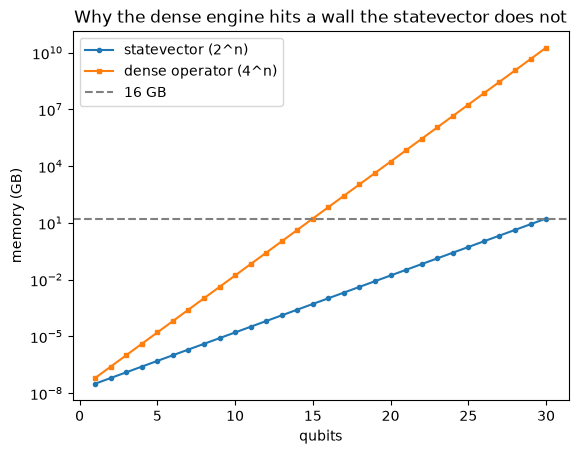
The reason is simple to picture. The statevector grows as 2^n. The dense operator grows as 4^n, its square. On a log scale they are two straight lines with different slopes, and the gap between them is the difference between roughly fifteen qubits and roughly thirty on the same machine.
ns = np.arange(1, 31)
statevector_gb = (2.0 ** ns) * 16 / 1e9
dense_gb = (2.0 ** ns) ** 2 * 16 / 1e9
fig, ax = plt.subplots()
ax.semilogy(ns, statevector_gb, marker="o", markersize=3, label="statevector (2^n)")
ax.semilogy(ns, dense_gb, marker="s", markersize=3, label="dense operator (4^n)")
ax.axhline(16, color="gray", linestyle="--", label="16 GB")
ax.set_xlabel("qubits")
ax.set_ylabel("memory (GB)")
ax.set_title("Why the dense engine hits a wall the statevector does not")
ax.legend()
plt.show()
A bonus: any gate, not just controlled ones
The dense apply could only do a single-qubit gate with some control qubits. The
tensor engine takes the full 2^k by 2^k matrix of any k-qubit gate and applies
it directly, so gates that were awkward before are now trivial. A SWAP exchanges
two qubits:
swap = np.array([[1, 0, 0, 0], [0, 0, 1, 0], [0, 1, 0, 0], [0, 0, 0, 1]], dtype=complex)
psi = np.zeros(8, dtype=complex)
psi[0b100] = 1                                              # |100>
out = apply_gate(psi, swap, [0, 2], 3)                     # swap qubit 0 and qubit 2
print("SWAP |100> on qubits 0,2 ->", format(int(np.argmax(np.abs(out))), "03b"))
SWAP |100> on qubits 0,2 -> 001
And a Toffoli (a NOT on the target only when both controls are 1), the three-qubit gate at the heart of reversible classical logic, is just its 8 by 8 matrix handed to the same function:
toffoli = embed(gates.X, 2, 3, controls=(0, 1))            # 8x8 Toffoli
psi = np.zeros(8, dtype=complex)
psi[0b110] = 1                                             # |110>: both controls set
print("Toffoli |110> ->", format(int(np.argmax(np.abs(apply_gate(psi, toffoli, [0, 1, 2], 3)))), "03b"))
Toffoli |110> -> 111
Honest limits
This is the standard exact statevector simulator, and it is what real tools use up to the point where exactness becomes impossible. The ceiling is now memory for the state, not the operator: 2^n complex numbers is about 16 GB at 30 qubits and a terabyte at 36, so a laptop tops out near 30. Past that you give something up. The research frontier uses tensor-network methods that stay cheap as long as the entanglement stays low, and approximate methods when it does not. We will not go there. Thirty qubits is plenty of room for the rest of this book.
Where this leaves us
We swapped the engine under the hood without changing a single result, and bought ourselves roughly fifteen extra qubits. That is the whole post: the same physics, computed the way it scales.
Everything up to here, including this faster engine, still represents a state as one vector with definite amplitudes. That picture has a hard edge, and we are about to walk off it. A real qubit is never alone; it is entangled with a world we do not track, and there is no single vector that describes it. The next post introduces the object that can: the density matrix.
Watch the Episode
This post is also a video episode: Many Qubits and Entanglement: Tensor Products, part of the series playlist.
Discussion