Shor's algorithm

This is the one everyone has heard of: the algorithm that factors integers in polynomial time and, if a big enough quantum computer is ever built, breaks RSA. It is also, pleasingly, mostly an application of the instrument we built last post. The quantum part of Shor’s algorithm is phase estimation. The rest is old number theory. The plan of attack is a chain of reductions: factoring reduces to finding the period of a function, the period is an eigenphase of a particular operator, and phase estimation reads eigenphases. Pull the chain and a factor falls out.

import math

import numpy as np
import matplotlib.pyplot as plt

from qfs.algorithms.shor import modmul_unitary, order_from_phase, shor_order, shor_factor

The classical half: periods give factors

None of this first part is quantum. Pick a number a coprime to N and look at its powers modulo N: a, a^2, a^3, .... They eventually cycle back to 1, and the smallest r with a^r = 1 (mod N) is the order of a. If r is even, then a^r - 1 = (a^{r/2} - 1)(a^{r/2} + 1) is a multiple of N, so unless a^{r/2} = -1 (mod N), the two factors a^{r/2} +/- 1 each share a real factor with N. A gcd finishes the job.

For N = 15 and a = 7, the order is r = 4 (we will find that quantumly in a moment). Here is the classical payoff, no quantum computer required.

a, N, r = 7, 15, 4
x = pow(a, r // 2, N)               # 7^2 mod 15 = 4
print(f"a^(r/2) mod N = {x}")
print(f"factors of {N}: gcd({x}-1, {N}) = {math.gcd(x - 1, N)}, gcd({x}+1, {N}) = {math.gcd(x + 1, N)}")

a^(r/2) mod N = 4
factors of 15: gcd(4-1, 15) = 3, gcd(4+1, 15) = 5

So the entire problem is: find the order r. Classically that is as hard as factoring. The quantum computer’s one job is to find it fast.

The quantum half: the period is an eigenphase

Consider the operator that multiplies by a modulo N: $U_a|x\rangle = |a x \bmod N\rangle$. It is a permutation, so it is unitary, and qfs builds it directly. Its eigenvalues are where the magic is. Because applying $U_a$ exactly r times returns every state to itself ($a^r = 1$), every eigenvalue is an r-th root of unity: $e^{2\pi i, s/r}$ for integer s. The eigenphases are multiples of 1/r.

U = modmul_unitary(7, 15, 4)   # third arg: 4 work qubits = ceil(log2(15)), not the order
phases = np.mod(np.angle(np.linalg.eigvals(U)) / (2 * np.pi), 1.0)
print("distinct eigenphases:", sorted(set(np.round(phases, 6))))

distinct eigenphases: [np.float64(0.0), np.float64(0.25), np.float64(0.5), np.float64(0.75)]

fig, ax = plt.subplots()
ax.hist(phases, bins=np.linspace(0, 1, 33))
for k in range(4):
    ax.axvline(k / 4, color="crimson", linestyle="--", linewidth=0.8)
ax.set_xlabel("eigenphase")
ax.set_ylabel("count")
ax.set_title("Eigenphases of 'multiply by 7 mod 15' land on multiples of 1/4")
plt.show()

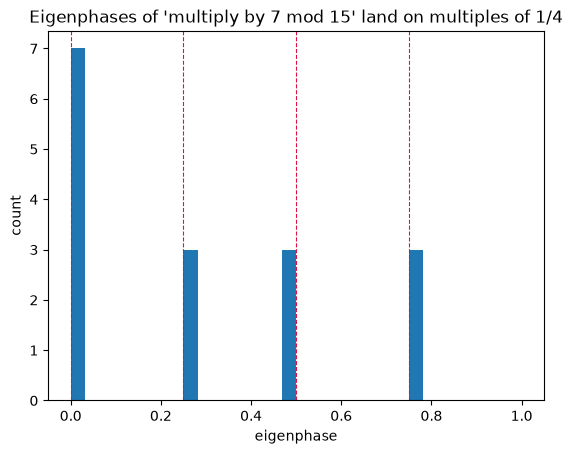
Every eigenphase sits on a red line, a multiple of 1/4. The denominator is the order. So if we could measure an eigenphase, a continued fraction would hand us r. That is exactly what phase estimation does, except for one obstacle: phase estimation needs an eigenstate to point at, and we do not know the eigenstates of $U_a$ without already knowing r.

The trick that makes Shor work: the plain computational state $|1\rangle$ is an equal superposition of $r$ of the eigenstates of $U_a$, one for each eigenphase $s/r$. So running phase estimation on $|1\rangle$ does not fail. It measures the eigenphase of a random one of them: a random $s/r$. shor_order runs phase estimation on $|1\rangle$, turns each measured phase into a candidate order by continued fractions, and keeps the ones that actually satisfy $a^r = 1$.

shor_order(7, 15, t=4, rng=np.random.default_rng(0))

4

Continued fractions: from a phase back to the period

A single run gives a phase like 0.25 or 0.75, a value s/r. The continued fraction of that phase, truncated to denominators below N, recovers r. Some runs are unlucky: a phase of 0.5 reduces to 1/2, suggesting r = 2, but 7^2 = 4 != 1 (mod 15), so that candidate is rejected and we try again.

for phi in (0.25, 0.5, 0.75):
    r_candidate = order_from_phase(phi, 15)
    verified = pow(7, r_candidate, 15) == 1
    print(f"measured phase {phi} -> candidate order {r_candidate}  (a^r = 1 mod N: {verified})")

measured phase 0.25 -> candidate order 4  (a^r = 1 mod N: True)
measured phase 0.5 -> candidate order 2  (a^r = 1 mod N: False)
measured phase 0.75 -> candidate order 4  (a^r = 1 mod N: True)

The whole thing

shor_factor runs the loop: pick bases, find an order, and reduce it to a factor by the classical gcd step. On N = 15 it returns 3 and 5.

shor_factor(15, t=4, rng=np.random.default_rng(0))

(3, 5)

An honest word about scale

This is a real, working Shor’s algorithm, and it is also stuck at N = 15. The reason is the simulator, not the algorithm. The register here is the counting qubits plus ceil(log2 N) work qubits, and our dense operators cost order $4^{\text{qubits}}$ in memory. Push to N = 21, where the order is 6 and the continued fractions actually have to work for their living, and the operators no longer fit. N = 15 is the standard textbook demonstration for exactly this reason: it is the largest case a naive simulator handles comfortably.

That limit is the hinge of the whole series. Everything so far has represented a state as one dense vector and a gate as one dense matrix, and we have now hit the wall that approach was always going to hit. The next post stops building algorithms and starts rebuilding the engine: a tensor-contraction simulator that applies a gate in time order $2^n$ instead of $4^n$, which is what real simulators do and what lets the qubit count grow. After that the series turns to the other thing the pure-state picture cannot express at all: open systems, noise, and the density matrix.

Where this leaves us

Shor’s algorithm is the payoff of the pure-state arc. Factoring became period finding, the period was an eigenphase, and phase estimation read it off, with the single clever step that $|1\rangle$ is a superposition of all the eigenstates so we never needed to know them. We built every piece from a length-two array upward, and watched 15 come apart into 3 and 5.

That closes the first half of the book. A state has been a single vector with definite amplitudes from the very first post. Real qubits are not like that: they leak into their surroundings, and to describe a qubit entangled with an environment we have stopped tracking, one vector is not enough. The second half starts there.