Many qubits, and entanglement

In post 0 a qubit was a unit vector in $\mathbb{C}^2$, and everything about it fit in a length-two array. One qubit is not where the interesting things are, though. This post adds the second qubit, and with it the one phenomenon that has no classical picture at all: entanglement. The good news is that it is still just a vector, now a slightly longer one, and the strangeness is a fact about how that vector does or does not factor.

import numpy as np

from qfs import gates
from qfs.statevector import StateVector
from qfs.circuit import Circuit
from qfs import viz

Two qubits live in a four dimensional space

The state space of $n$ qubits is the tensor product of $n$ copies of $\mathbb{C}^2$, which is $\mathbb{C}^{2^n}$. Two qubits give $\mathbb{C}^4$, a length-four vector. The basis states are the four bit strings, $|00\rangle$, $|01\rangle$, $|10\rangle$, $|11\rangle$, and qfs indexes them in that order (big-endian: qubit 0 is the leftmost, most significant bit).

A fresh two-qubit register is $|00\rangle$.

sv = StateVector(2)
sv.amps  # length 4: [|00>, |01>, |10>, |11>]

array([1.+0.j, 0.+0.j, 0.+0.j, 0.+0.j])

Independent qubits: the state factors

If two qubits are prepared independently, the joint state is the tensor product of the two single-qubit states. Put each qubit into $|+\rangle$ with a Hadamard, and the joint state is $|+\rangle \otimes |+\rangle$: all four amplitudes equal.

sv = StateVector(2).apply(gates.H, 0).apply(gates.H, 1)
sv.amps

array([0.5+0.j, 0.5+0.j, 0.5+0.j, 0.5+0.j])

There is a concrete fingerprint of a state that factors. If $|\psi\rangle = (a_0|0\rangle + a_1|1\rangle) \otimes (b_0|0\rangle + b_1|1\rangle)$, then the four amplitudes are $a_0 b_0,\ a_0 b_1,\ a_1 b_0,\ a_1 b_1$, and so

Both sides equal $a_0 a_1 b_0 b_1$. A product state always satisfies this.

a = sv.amps
np.isclose(a[0] * a[3], a[1] * a[2])  # True: this state factors

np.True_

CNOT, and a state that does not factor

Now entangle them. Put qubit 0 into a superposition, then apply a controlled-NOT with qubit 0 as control and qubit 1 as target. CNOT flips the target exactly when the control is 1. In qfs a control is just an extra argument to apply.

bell = StateVector(2).apply(gates.H, 0).apply(gates.X, 1, controls=(0,))
bell.amps  # (|00> + |11>)/sqrt(2)

array([0.70710678+0.j, 0.        +0.j, 0.        +0.j, 0.70710678+0.j])

This is a Bell state, $\frac{1}{\sqrt 2}(|00\rangle + |11\rangle)$. Run the same factorization check and it fails.

a = bell.amps
print("amp00 * amp11 =", a[0] * a[3])
print("amp01 * amp10 =", a[1] * a[2])
np.isclose(a[0] * a[3], a[1] * a[2])  # False: no product of single-qubit states gives this

amp00 * amp11 = (0.4999999999999999+0j)
amp01 * amp10 = 0j





np.False_

That failure is the whole content of entanglement. There is no pair of single-qubit states whose tensor product is this vector. So there is no answer to the question “what state is qubit 0 in.” Qubit 0 does not have a state of its own here. Only the pair does. Nothing was hidden and nothing travels faster than light. The joint vector simply does not split into a part for each qubit.

What entanglement does to measurement

The consequence you can watch: measure qubit 0 of the Bell state, then qubit 1, and they always agree. The first measurement collapses the joint vector onto the slice consistent with its outcome, and in this state that slice has already fixed the second qubit. Measuring the first qubit is measuring the second.

rng = np.random.default_rng(0)
results = []
for _ in range(20):
    sv = StateVector(2, rng=rng).apply(gates.H, 0).apply(gates.X, 1, controls=(0,))
    results.append((sv.measure(0), sv.measure(1)))

print("(qubit0, qubit1) outcomes:", results)
print("always equal:", all(b0 == b1 for b0, b1 in results))

(qubit0, qubit1) outcomes: [(0, 0), (1, 1), (0, 0), (0, 0), (0, 0), (0, 0), (0, 0), (0, 0), (0, 0), (1, 1), (1, 1), (0, 0), (0, 0), (0, 0), (0, 0), (0, 0), (1, 1), (0, 0), (1, 1), (0, 0)]
always equal: True

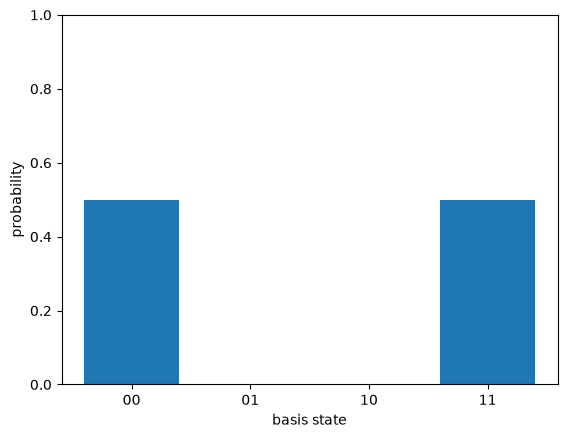
Sampling many copies of the un-measured Bell state shows the other half of the picture: only $00$ and $11$ ever appear, each about half the time, and $01$ and $10$ never do. The correlation is built into the amplitudes.

counts = StateVector(2, rng=np.random.default_rng(1)).apply(gates.H, 0).apply(gates.X, 1, controls=(0,)).sample(2000)
print(counts)
_ = viz.plot_probabilities(StateVector(2).apply(gates.H, 0).apply(gates.X, 1, controls=(0,)))

{'11': 998, '00': 1002}

The same thing, as a circuit

Writing out apply calls gets tedious. qfs has a small Circuit type that records a sequence of gates and runs them on a fresh register. The Bell state is a Hadamard followed by a CNOT, and it reads that way.

state = Circuit(2).h(0).cnot(0, 1).run()
state.amps

array([0.70710678+0.j, 0.        +0.j, 0.        +0.j, 0.70710678+0.j])

Where this leaves us

Adding a qubit doubled the length of the vector and bought us a genuinely new thing: states that do not factor. Entanglement is not a mechanism, it is the absence of one, the failure of the joint state to come apart into independent pieces. We built it with one CNOT and watched it force two measurements to agree.

Two qubits is also enough to do something a classical computer cannot do as cheaply. In the next post we build actual circuits, Deutsch-Jozsa and Bernstein-Vazirani, and see interference, where amplitudes add and cancel, do real computational work.