What is a qubit?

I wanted to understand quantum computing properly, which for me means building the thing rather than driving a framework that does the linear algebra in the basement and hands back an answer. So this series builds a simulator from nothing, in Python, on top of NumPy, and writes down what falls out along the way. The code lives in a small package called qfs. Each post adds one piece.

The encouraging part, and the reason a from-scratch approach is even sane here: a single qubit is a tiny object. It is a unit vector in a two dimensional complex space. That is the entire definition. Everything that gets described as spooky (superposition, the Bloch sphere, measurement collapse) is something you can watch happen inside a length-two array. Nothing is hidden. By the end of this post we will have looked at all three directly.

import numpy as np

from qfs import gates
from qfs.statevector import StateVector
from qfs import viz

The state is a vector

A qubit state is a vector in $\mathbb{C}^2$:

The two basis vectors $|0\rangle = (1, 0)$ and $|1\rangle = (0, 1)$ are the classical bit values. The numbers $\alpha$ and $\beta$ are amplitudes. They are complex, and they are not probabilities. The probabilities come later, when we measure, and they are the squared magnitudes of the amplitudes. The normalization constraint $|\alpha|^2 + |\beta|^2 = 1$ is just the statement that those probabilities have to sum to one.

In qfs a state is a StateVector. A fresh one starts in the ground state $|0\rangle$.

psi = StateVector(1)
psi.amps

array([1.+0.j, 0.+0.j])

That array is the state. amps[0] is the amplitude of $|0\rangle$, amps[1] the amplitude of $|1\rangle$. The probabilities are the squared magnitudes:

psi.probabilities()

array([1., 0.])

Gates are unitary matrices

A quantum gate on one qubit is a $2 \times 2$ matrix. It has to be unitary, meaning $U^\dagger U = I$, for one concrete reason: the state is required to stay a unit vector (the probabilities must keep summing to one), and unitary matrices are exactly the ones that preserve length. So the constraint is not a rule imposed from outside. It is the only kind of matrix that keeps a valid state valid.

Three gates are enough to get started. X is the bit flip (the quantum NOT). Z leaves $|0\rangle$ alone and flips the sign of $|1\rangle$. H, the Hadamard, is the one that builds a superposition.

# X flips |0> to |1>
StateVector(1).apply(gates.X, 0).amps

array([0.+0.j, 1.+0.j])

# H takes |0> to an equal superposition, usually written |+>
StateVector(1).apply(gates.H, 0).amps

array([0.70710678+0.j, 0.70710678+0.j])

Superposition is just a vector that is not on an axis

That last state, $\frac{1}{\sqrt{2}}(|0\rangle + |1\rangle)$, is “superposition.” It is worth saying plainly what it is and is not. It is a unit vector that does not point along either basis axis. Nothing is in two places. The qubit is not secretly 0 and 1 at the same time in any classical sense. There are just two amplitudes, both nonzero, and they are bookkeeping for what happens when this state interferes with itself or gets measured.

Apply H twice and the two halves interfere back into the state you started with. That cancellation is the whole game later, when algorithms arrange for the wrong answers to cancel and the right ones to add.

StateVector(1).apply(gates.H, 0).apply(gates.H, 0).amps

array([1.+0.j, 0.+0.j])

The Bloch sphere: the geometry of one qubit

A single qubit has more structure than a list of two complex numbers lets you see at a glance. Two complex numbers are four real numbers, the normalization removes one, and an overall phase that has no observable effect removes another. What is left is two real degrees of freedom, which is the surface of a sphere. Every pure single-qubit state is a point on it. This is the Bloch sphere.

The three coordinates of that point are the expectation values of the Pauli observables, $\langle X \rangle$, $\langle Y \rangle$, and $\langle Z \rangle$. $|0\rangle$ sits at the north pole, $|1\rangle$ at the south, and equal superpositions like $|+\rangle$ live on the equator. Unequal superpositions sit between the poles, closer to whichever basis state carries more amplitude.

viz.bloch_vector(StateVector(1))                    # |0> -> north pole

array([0., 0., 1.])

viz.bloch_vector(StateVector(1).apply(gates.X, 0))  # |1> -> south pole

array([ 0.,  0., -1.])

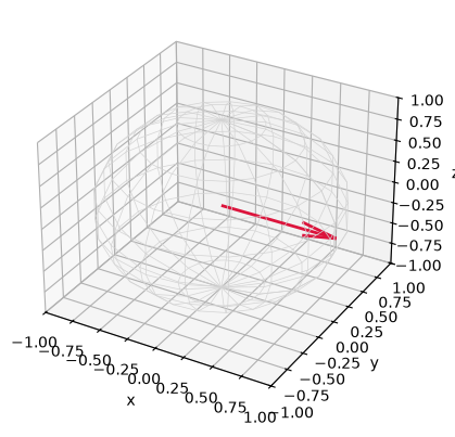
viz.bloch_vector(StateVector(1).apply(gates.H, 0))  # |+> -> on the equator

array([1., 0., 0.])

# bind to _ so the figure renders once (the inline backend), not twice
_ = viz.plot_bloch(StateVector(1).apply(gates.H, 0))

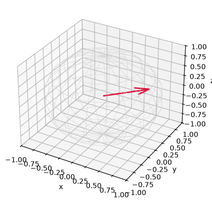
Once you have the sphere, the rotation gates stop being abstract. Ry(theta) rotates the state by an angle theta around the y axis. Dial theta and the point slides from the north pole down toward the equator and on to the south. Here is a state a third of the way around.

psi = StateVector(1).apply(gates.Ry(np.pi / 3), 0)
print("bloch vector:", viz.bloch_vector(psi))
print("amplitudes:  ", psi.amps)
_ = viz.plot_bloch(psi)

bloch vector: [0.8660254 0.        0.5      ]
amplitudes:   [0.8660254+0.j 0.5      +0.j]

Measurement: the one irreversible step

Everything so far is reversible. Gates are unitary, so you can always undo them. Measurement is the exception, and it is where the probabilities finally show up.

The Born rule: the probability of outcome $b$ is $|\alpha_b|^2$. Measuring does two things. It samples an outcome according to those probabilities, and then it collapses the state to be consistent with what it saw. After you measure a qubit and get 0, the state is exactly $|0\rangle$. The other amplitude is gone.

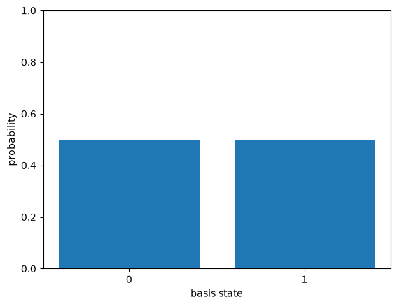
Start with $|+\rangle$, where the two outcomes are equally likely.

psi = StateVector(1).apply(gates.H, 0)
psi.probabilities()

array([0.5, 0.5])

Sampling many shots of a freshly prepared $|+\rangle$ gives roughly half zeros and half ones. (sample does not collapse the stored state, it just draws outcomes from the current probabilities, which is what a real run of many identical preparations would give you.)

shots = StateVector(1, rng=np.random.default_rng(0)).apply(gates.H, 0).sample(1000)
shots

{'1': 527, '0': 473}

_ = viz.plot_probabilities(StateVector(1).apply(gates.H, 0))

A single measure is the irreversible one. It returns a bit and leaves the state collapsed onto the matching basis state. Run the next cell a few times with different seeds and you will see the outcome flip between 0 and 1, but the post-measurement state is always a definite basis state, never the superposition you started from.

psi = StateVector(1, rng=np.random.default_rng(2)).apply(gates.H, 0)
outcome = psi.measure(0)
print("measured:", outcome)
print("state after measurement:", psi.amps)

measured: 1
state after measurement: [0.+0.j 1.+0.j]

Where this leaves us

That is a qubit, in full. A unit vector in $\mathbb{C}^2$. Gates are unitary rotations of that vector, and the Bloch sphere makes the rotations literal. Measurement is sampling by the Born rule followed by collapse. No piece of that needed a framework or a quantum computer, just a length-two complex array and the constraint that it stay normalized.

One qubit is not where the interesting things are, though. The moment you have two qubits, you can write down states that do not factor into a separate state for each qubit. There is no answer to “what is qubit 0 doing” on its own. That failure to factor is entanglement, and it is the next post, where we generalize the StateVector to many qubits and build the first Bell state.